 Embedded HandbookApps
85. TinyML: machine learning on a microcontroller
TinyML is machine learning right where the data is born: on a microcontroller next to the sensor, drawing on the order of milliwatts. The device does not send the raw signal to the cloud; it decides by itself: was the keyword spoken, which gesture was made, is the bearing wearing out. This is faster, needs no network and keeps the data on the device.
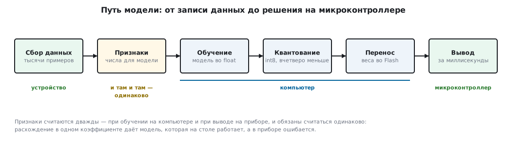
The main thing to understand: on a microcontroller the model does not learn, it only runs. You train it on a computer, then shrink it and put it into Flash as an ordinary array of numbers. This section walks the whole path on a small example — from the data to integer inference in C — and every number is verified by a build and by calculation.
Terms used in the documentation
Term Meaning machine learning, model learning from data; the trained result feature, feature vector a number the model decides by; a set of them training / inference fitting the model / running it on new data supervised / unsupervised learning with known answers / without answers classification, anomaly detection choosing a class; finding the unusual train / test split data for training and data held back for testing quantization, scale, zero point storing reals as integers; step; integer for zero multiply–accumulate (MAC) multiply and add to a running sum keyword spotting, wake word recognizing a spoken keyword spectrogram, MFCC spectra over time; mel-frequency cepstral coefficients autoencoder, k-means a network that rebuilds its input; clustering around centers
85.1 How it works
| Step | Where | What you get |
|---|---|---|
| data collection | device, recording | thousands of labeled examples |
| features | computer and device — identically | the numbers the model decides by |
| training | computer | a float model |
| quantization | computer | an int8 model, four times smaller |
| transfer | computer → firmware | an array of weights in Flash |
| inference | microcontroller | a decision in milliseconds |
Supervised learning is when the correct answer is known for each example: "this is the word 'yes'", "this is wear". Unsupervised is when there are no answers and the model looks for patterns by itself; this is how anomalies are found.
Features can be binary (yes/no), categorical (color, type), ordinal (a rating on a scale) and quantitative (a measured value). A quantitative feature does not have to be unbounded — a temperature within its allowed limits is quantitative too; but a rating "bad — good — excellent" is written as numbers, yet adding them makes no sense: it is an order.
Four typical TinyML tasks and their data:
| Task | Sensor | How much data |
|---|---|---|
| keyword | microphone | 16000 samples per second |
| gesture | accelerometer | hundreds of samples per second |
| wear, anomaly | vibration sensor | thousands of samples per second |
| object in the frame | camera | tens of kilobytes per frame |
85.2 Features: not the raw signal but its essence
Audio for speech recognition is sampled at 16 kHz — enough for a bandwidth of up to 8 kHz. One second of such audio in int16 is 32000 bytes, more than the whole RAM of an F103C8 (20 KB, section 80.1). So the signal is not stored whole; it is cut into windows of 30 ms with a step of 20 ms, and each window is immediately turned into features:
- the fast Fourier transform gives the spectrum of the window — which mix of frequencies it consists of; a series of spectra in a row is a spectrogram;
- the spectrum is folded into 13 mel-frequency cepstral coefficients (MFCC): they emphasize the low frequencies, which the ear tells apart better.
One second of audio is 49 windows of 13 coefficients, 637 features instead of 16000 samples. Whether the word is said loudly or quietly, the features look alike — that is why they are computed.
The rule that projects break on: features on the device must be computed exactly as during training — the same windows, the same constants, the same scale. A model trained on one kind of features that receives another answers with garbage, and no accuracy on the computer will show it. Simple features — mean, moving average, peak-to-peak range — are computed by the filters from section 81.
85.3 The model in memory: why int8
A small network for keywords: 637 features → 32 neurons → 3 answers. It has 20515 parameters:
| Storage | Size | F103C8 (Flash 64 KB) |
|---|---|---|
| float, 4 bytes | 82060 bytes | does not fit |
| int8, int32 biases | 20620 bytes | fits |

"Fits" here refers to the weights. The firmware needs two more things. Code
that runs the model: your own loop, as in 85.5, is hundreds of bytes, while
TensorFlow Lite for Microcontrollers, even with a single FullyConnected
operation, takes about 21 KB of Flash (armclang -Os, Cortex-M3).
Together with the weights that is 41 KB out of 64 — about a third is left for the rest
of the firmware. And RAM for intermediate results: for this network that is the 637-byte input,
32 bytes of the first layer and 3 answers, plus the audio window buffers. Libraries
call this area the working memory (tensor arena) and require you to allocate it
in advance as one array; how much a particular model needs is estimated by
STM32Cube.AI (85.8).
Quantization replaces each real number with an integer from −128 to 127: x ≈ scale · (q − zero point).
/* ── квантование: x ≈ scale · (q − zero) ── */
int8_t quantize(float x, float scale, int zero)
{
    long q = lroundf(x / scale) + zero;
    if (q > 127)
        q = 127;
    if (q < -128)
        q = -128;
    return (int8_t)q;
}
The error is no more than half a step: in the check with a step of 1/127 on the interval from −1 to 1 it came to 0.003937, exactly 1/254. This usually hardly hurts the model — below you can see by how much.
85.4 The cost of inference and what Cortex-M computes it with
One inference of this network is 20480 multiply–accumulates, one for each weight. How the core executes them is visible in the machine code:
| Core | Instructions per multiply–accumulate |
|---|---|
| Cortex-M0 | two: muls and adds |
| Cortex-M3 | one: mla |
| Cortex-M4, compiler code | one: smlabb (a DSP instruction, but one multiply at a time) |
| Cortex-M4, CMSIS-NN library | smlad — two multiplies per instruction, sxtb16 unpacks the bytes |
The compiler did not insert the packed instruction by itself: a plain loop on the M4 is
smlabb, one multiply per element. The CMSIS-NN kernel for the M4 has 42
smlad instructions and as many sxtb16, while the same kernel for the M3 builds with mla only.
That is why on an F407 the neural network is computed with the library, not with your own loop.
Floating-point arithmetic is the same story: the square root in the anomaly detector from
85.6 on an M4 with an FPU is a single vsqrt.f32 instruction; on an M3 it is a call to a library
function (section 69).
85.5 The whole path on a small example
The task: tell a healthy bearing from a worn one by vibration. Two features per window: the RMS value of the vibration and the share of energy in the upper frequency band. On the computer there are 2000 examples: 1500 for training, 500 for testing, which the model has never seen.
Training. Logistic regression: a weighted sum of the features plus a bias; the decision is made by the sign. Gradient descent in Python gave weights of 2.392 and 4.215 and a bias of 0.781.
Quantization. Features and weights go to int8, each with its own scale; the bias goes to
int32 in units of "feature scale × weight scale". The quantization here is symmetric:
the zero point of the features and weights is zero, so dot_s8 simply
multiplies the codes. With a non-zero zero point, you first subtract it from each
code (or fold a correction into the bias in advance), otherwise the sum drifts. The weights became the integers 72 and 127,
the bias 1015. The script writes them into a header — this is how the model
gets into the firmware, as an array in Flash:
#define ML_N 2
static const int8_t ML_W[ML_N] = {72, 127};
#define ML_B (1015)
Inference on the microcontroller — entirely in integers:
/* ── скалярное произведение int8 с накоплением в int32 ── */
int32_t dot_s8(const int8_t *a, const int8_t *b, int n)
{
    int32_t acc = 0;
    for (int i = 0; i < n; i++)
        acc += (int32_t)a[i] * b[i];
    return acc;
}

/* ── классификатор: знак w·x + b целиком в целых числах ── */
int ml_classify_q(const int8_t *xq)
{
    return dot_s8(ML_W, xq, ML_N) + ML_B > 0;
}
Result on 500 test examples:
| Model | Correct |
|---|---|
| float on the computer | 494 of 500 |
| int8 in C | 494 of 500 |
| float and int8 answers matching | 500 of 500 |
Quantization did not cost a single correct answer. The int8 inference in C gave exactly
the same result as the integer calculation in Python — this is the
proof that the model was transferred without errors. The code is built with armclang for
Cortex-M0, M3 and M4 without warnings.
85.6 Anomalies: learn only what is normal
Wear, leaks and breakdowns share a difficulty: there are few examples of faults, and thousands of ways to break. You can collect data on "how a machine breaks" only by breaking machines. The way out is to teach the model only what is normal and treat everything that does not look like it as an anomaly.
The simplest option needs no neural network: compute the mean and spread of the signal on the fly and raise an alarm when a sample moves away from the mean by more than a set number of sigmas. Welford's algorithm does this in a single pass, without storing the samples:
typedef struct {
    uint32_t n;
    float mean;
    float m2;       /* сумма квадратов отклонений от среднего */
} welford_t;

void welford_add(welford_t *w, float x)
{
    w->n++;
    float d = x - w->mean;
    w->mean += d / (float)w->n;
    w->m2 += d * (x - w->mean);
}

/* На сколько сигм x отстоит от накопленной нормы */
float welford_z(const welford_t *w, float x)
{
    if (w->n < 2)
        return 0.0f;
    float var = w->m2 / (float)(w->n - 1);
    return var > 0.0f ? (x - w->mean) / sqrtf(var) : 0.0f;
}
In the check, the detector learned on 1000 samples of normal data with a 4σ threshold: false alarms — zero, and a 6σ shift of the mean was caught on the very first sample. The state is 12 bytes.
For multidimensional data the same principle is taken further: k-means remembers the centers of groups of normal examples and measures the distance to the nearest one; an autoencoder — a neural network trained to rebuild the normal signal through a narrow bottleneck — rebuilds anomalies poorly, and a large reconstruction error raises the flag. The key point: you stop training the detector as soon as it has started working, otherwise it gradually accepts the anomaly as normal.
85.7 Images: why not a sliding window
The most direct way to find an object in a frame is to slide a window over it and ask the model about each position. A 48×48 window with a step of 16 over a 160×120 frame is 40 positions; at 100 ms per inference that is 4 seconds per frame. So on a microcontroller you use a low resolution and networks that in a single pass give both the class and the location of the object, or first pick out "interesting" regions with a simple algorithm and classify only those.
85.8 Tools
- TensorFlow Lite for Microcontrollers — converts a trained model into an array and runs it on the device;
- CMSIS-NN — fast neural network kernels for Cortex-M (85.4); other inference libraries rely on them too;
- STM32Cube.AI — converts models for STM32 and estimates memory and inference time on a specific chip;
- online services that collect data from a phone or a board, train the model and hand out ready code — handy for a first prototype.
85.9 Responsibility
A model always makes mistakes — the question is how often and what it costs. A false alarm about an engine failure means stopping the line; a missed one means an accident. The threshold is chosen by the cost of an error, and accuracy is measured on data from real conditions: with noise, echo, other voices. A sensor that is always listening or watching collects data about people: protect it like any other data (section 37.4), or better not store it at all — the decision is made on the spot and only the result leaves the device.
85.10 Pitfalls
In the lab the model recognizes the word, outdoors it does not. The data was collected in silence; you need noise, echo, different voices and distances.
Accuracy on the computer is 99%, on the device it is random. The features on the device are computed differently than during training.
The test showed 100%. It was tested on the same data the model was trained on.
The model does not fit into Flash. The weights are in float; after quantization to int8 they are four times smaller.
After quantization the answers "drifted". The scale was not chosen by the range of the data, and large values hit ±127.
Inference takes seconds. Your own loop instead of CMSIS-NN on the M4, a network too big for the chip, a sliding window over the frame.
Floating-point calculations are slow. The M0 and M3 have no FPU — everything goes through the library.
The anomaly detector stopped firing. It kept learning and accepted the fault as normal.
85.11 Summary
- On a microcontroller the model only runs; it is trained on a computer, shrunk and put into Flash as an array.
- Features are computed identically during training and on the device; one second of 16 kHz audio is 32000 bytes, and it gives 637 features.
- int8 is four times smaller than float: a network of 20515 parameters is 82060 bytes in float and 20620 in int8; the quantization error is no more than half a step.
- Cortex-M0 multiplies and adds with two instructions, M3 with one
mla, M4 in CMSIS-NN withsmlad, two multiplies per instruction. - The whole example: 494 of 500 both in float and in int8; all 500 answers matched, the C inference matched the Python calculation.
- Anomalies are found by learning only what is normal: mean and spread on the fly take 12 bytes and gave not a single false alarm on 1000 samples.
Next: section 86 "Network types and core technologies".