 Embedded HandbookApps
162. Single-supply path to the ADC: y = m·x + b
A sensor gives its own range, and the ADC expects 0…3.3 V. Between them there is almost always the same task: stretch and shift the signal so that it fills the scale but does not hit the rails. On a single supply this task has exactly four variants — by the signs of the slope and the offset — and each has its own circuit built on one amplifier.
Terms used in the documentation
Term Meaning single supply one supply rail plus ground, no negative rail transfer function output as a function of input gain, slope how much the output changes per unit of input offset a constant shift of the output reference voltage a fixed voltage the circuit is referred to voltage divider two resistors that scale a voltage down Thevenin equivalent a source with a series resistance that replaces a network output swing how close the output gets to the rails headroom margin left to the supply rail resistor tolerance allowed deviation of a resistor from its nominal value worst-case analysis calculation for the worst combination of tolerances E24 series the standard series of 24 nominal values per decade
162.1 Two points, and the circuit is chosen
The output of a linear circuit on one amplifier is always a straight line y = m·x + b.
Two points define it completely: the low end of the sensor range must
land slightly above ADC zero, the high end slightly below 3.3 V. A margin of 0.1 V on
each side is needed because the output does not reach the rails even on a part
with full swing, and the sensor and resistors have spread (162.6).
m = (y2 − y1) / (x2 − x1), b = y1 − m·x1
The signs of m and b choose the circuit:
| b > 0 | b < 0 | |
|---|---|---|
| m > 0 | A: non-inverting, offset added at "+" | B: non-inverting, bottom leg to a reference |
| m < 0 | C: inverting, "+" at a reference | D: inverting, offset from the supply into "−" |
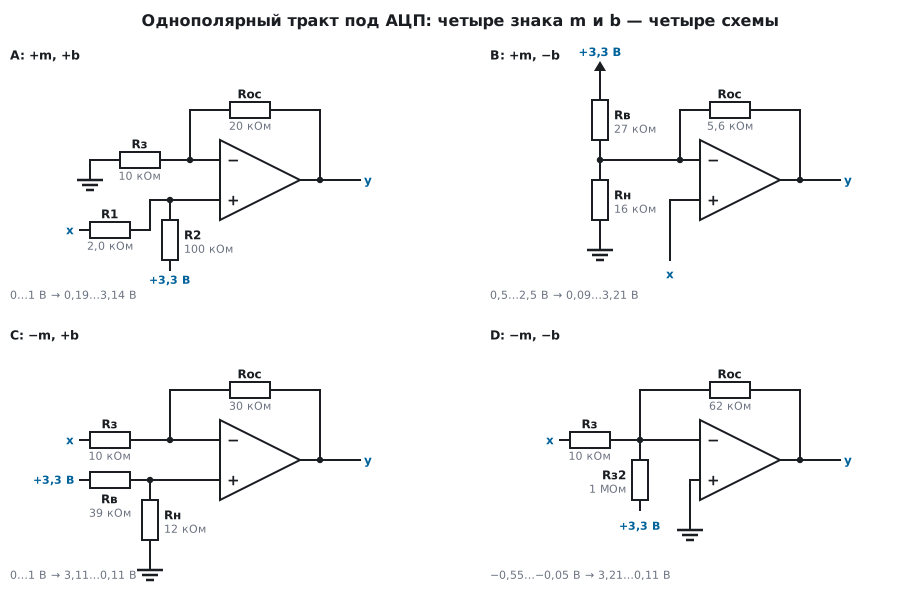
All four circuits below are calculated with E24 values and checked with a model in ngspice (an amplifier with 1 MHz bandwidth, output reaching within 0.05 V of the rails).
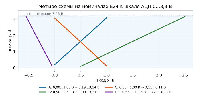
162.2 Case A: +m, +b
Sensor 0…1 V → 0.2…3.1 V: m = 2.9, b = 0.2. The input and the supply
are summed by a divider at the non-inverting input, followed by non-inverting
gain G = 1 + Rf/Rg:
y = G · (x · R2/(R1 + R2) + Vs · R1/(R1 + R2))
where R1 is on the input side and R2 on the supply side. From this G = m + b/Vs
and the input share k = m/G. The node at "+" must not be in the megohms (pickup,
input current — section 56.4), so R2 is chosen as 100 kΩ and R1 is calculated:
it comes out at 2.09 kΩ → 2.0 kΩ; Rf/Rg = 20 kΩ / 10 kΩ.
Model: 0.19 V at x = 0 and 3.14 V at x = 1 V — instead of the target 0.2 and 3.1: this is how the nominal values rounded.
The sensor now drives R1 + R2 = 102 kΩ to the supply: at x = 0, 32 µA flows into its output. Its output resistance adds to R1, and the offset is proportional to R1: 20 Ω adds 1 % to b, 200 Ω adds 10 %. A sensor with an output resistance of hundreds of ohms (a divider, a thermistor) is either included in the calculation of R1, or a follower is placed in front of the circuit.
162.3 Case B: +m, −b
Sensor 0.5…2.5 V → 0.1…3.2 V: m = 1.55, b = −0.675. A non-inverting
amplifier whose bottom leg goes not to ground but to a reference:
y = x · (1 + Rf/Rg) − Vref · Rf/Rg
The reference and the bottom leg come from one divider: by Thevenin it is a source
Vref = Vs · Rbot/(Rtop + Rbot) with a resistance of Rtop ∥ Rbot. The values are chosen so
that this resistance is exactly Rg: 27 kΩ and 16 kΩ give 1.23 V and
10.05 kΩ, Rf = 5.6 kΩ. A separate Rg resistor is not needed, and the divider
does not need a buffer.
Model: 0.09 V at 0.5 V and 3.21 V at 2.5 V.
162.4 Case C: −m, +b
Sensor 0…1 V → 3.1…0.1 V, a "reversed" scale: m = −3. An inverting
amplifier with the non-inverting input at a reference:
y = −x · Rf/Rg + Vref · (1 + Rf/Rg)
Rf/Rg = 30 kΩ / 10 kΩ, the reference is a 39 kΩ / 12 kΩ divider, 0.78 V.
No current flows into the "+" input, so the resistance of this divider
does not affect the gain.
Model: 3.11 V at x = 0 and 0.11 V at x = 1 V.
162.5 Case D: −m, −b
The input is below ground — for example, a shunt in the negative lead: −0.55…−0.05 V →
3.2…0.1 V, m = −6.2, b = −0.21. An inverting amplifier, "+" at
ground, the offset is a current from the supply through Rg2 into the inverting input:
y = −x · Rf/Rg − Vs · Rf/Rg2
Rf/Rg = 62 kΩ / 10 kΩ, Rg2 = 1 MΩ.
Model: 3.21 V at −0.55 V and 0.11 V at −0.05 V. The inverting input sits at zero here — the amplifier must work with its input right at the bottom rail; check this in the documentation.
162.6 Resistor tolerances: the worst case
Nominal values are not yet a circuit. Recalculating case B for all eight combinations of the extreme values of the three resistors:
| Tolerance | Slope m | Offset b | Bottom of scale | Top of scale |
|---|---|---|---|---|
| 5 % | −3.4 … +3.8 % | −9.5 … +10.5 % | 0.03 … 0.15 V | 3.13 … 3.30 V |
| 1 % | ±0.7 % | ±2.0 % | 0.08 … 0.11 V | 3.19 … 3.23 V |
| supply ±2 %, exact resistors | 0 | ±2.0 % | 0.08 … 0.11 V | 3.20 … 3.22 V |
With 5 % resistors the offset wanders by ten percent, and the top of the scale in the worst combination needs 3.30 V — the output runs into its 3.25 V ceiling at the rail, and the top ADC codes are lost. With 1 % the path fits within the 0.1 V margin.
In all four circuits the offset b is taken from the supply, and the regulator tolerance goes into it in full: ±2 % on the supply is the same ±2 % on the offset as with 1 % resistors (the "supply" row of the table). In case C the whole offset of 3.11 V comes from the supply, and there that is already ±62 mV. If the ADC measures from the same rail, the offset in codes cancels — it is proportional to the supply — but the slope changes by the same ±2 %: the sensor voltage does not depend on the supply. If the ADC has its own reference, the supply tolerance is added to the resistor tolerances. The amplifier's offset voltage appears at the output multiplied by 1 + Rf/Rg: in case B by 1.56 times, in case D by 7.3 times (there Rg means Rg ∥ Rg2).
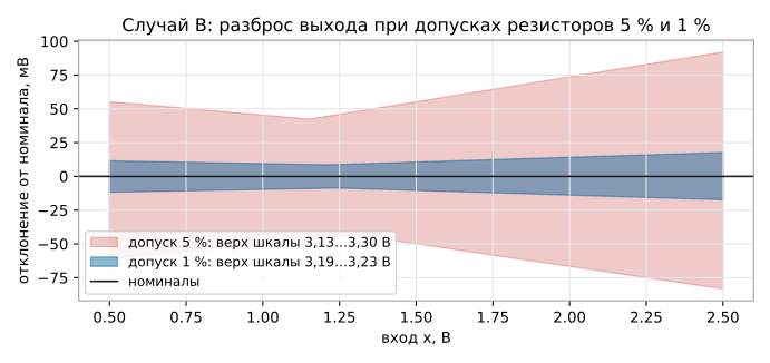
Hence the rule: either 1 % resistors, or a larger margin at the rails, or a two-point calibration in software.
162.7 Pitfalls
The signal at the top of the ADC range is "clipped". The output does not reach the rail; the calculation was done without margin, or on nominal values rather than the worst combination of tolerances.
Circuit B gives the wrong slope. The resistance of the reference divider was not taken into account: it is in series with the bottom leg.
The offset "drifts" with supply noise. The reference is taken straight from
the supply; a divider without a capacitor passes the ripple to the output,
multiplied by Rf/Rg.
Case D does not work on an ordinary amplifier. The input must work at the bottom rail. Amplifiers whose input range does not reach it are not suitable — for example, the TL07x on a single supply; the LM358/LM324 (input down to ground) and amplifiers with rail-to-rail input are suitable.
A megohm node at "+" picks up interference. In case A the divider resistances are chosen in the hundreds of kilohms, not megohms.
162.8 Summary
- A linear path on one amplifier is a straight line
y = m·x + b; two points (with a 0.1 V margin at the rails) set m and b, and the signs pick one of four circuits. - A: 0…1 V → 0.19…3.14 V with 2.0 kΩ / 100 kΩ and ×3; B: 0.5…2.5 V → 0.09…3.21 V with a 27 kΩ / 16 kΩ divider that gives both the 1.23 V reference and the 10.05 kΩ bottom leg.
- C: 0…1 V → 3.11…0.11 V, inverting ×−3 with a 0.78 V reference; D: −0.55…−0.05 V → 3.21…0.11 V, ×−6.2 and an offset from the supply through 1 MΩ.
- 5 % resistors shift b by 10 % and push the top of the scale to 3.30 V — past the rail; 1 % keep it within 3.19…3.23 V.
Next: section 163 "Stability: phase margin and capacitive load".