 Embedded HandbookApps
36е. Oscilloscope, part 3: cursors, automatic measurements, math and FFT
The first two parts are about how a signal gets into memory (36г) and how to catch the right moment (36д). This one is about getting a number out of the record: how many volts, how many microseconds, what frequency, how much energy, what is in the spectrum. The instrument computes fast and shows the result with four digits, and that is exactly why it is easy to trust. But every number is computed by a rule: where the top is, where the base is, which threshold defines an edge, which piece of the record is used. If the rule does not fit the signal, the instrument honestly gives a wrong number.
For each function: what it is, what it is for, what you see, a typical mistake and a case from the life of a microcontroller board. The order: cursors, automatic measurements by group, statistics and histogram, the built-in voltmeter and frequency counter, channel math, FFT and the Bode plot.
The examples use the author's instrument, a RIGOL DHO900: menu items are named in English as they appear on the screen, and the figures come from its documents. The effects themselves are common to any digital oscilloscope; whatever applies only to the DHO900 is marked as such.
Sources: RIGOL DHO900 User Guide (Books/DHO900_UserGuide_EN.pdf; pages
here and below are PDF file pages): pp. 128–148 — math (arithmetic,
functions, FFT, logic, filters), pp. 149–162 — automatic measurements,
thresholds, statistics, pp. 163–171 — cursors, pp. 172–176 — voltmeter and
frequency counter, pp. 181–185 — histogram, pp. 194–200 — Bode plot; RIGOL
DHO900 Datasheet (Books/dho900-datasheet.pdf): pp. 10–11 — gain, offset
and time interval accuracy, p. 16 — cursors and measurements, p. 17 —
math and FFT, p. 18 — histogram, p. 19 — Bode, p. 22 — voltmeter and
frequency counter. All calculated figures come from a run of
_verify/scope36e/model36e.py (Python 3.11 and numpy in the stm-lab:1 container).
What it is called in the documentation
Original Meaning cursor: Manual, Track, XY; AX, BX, ∆X, 1/∆X, ∆Y cursors: manual, tracking, XY; readouts and differences auto measurement; Indicator automatic measurement; cursors showing where it was taken Vtop, Vbase, Vamp; Vmax, Vmin, Vpp top, base, amplitude; maximum, minimum, peak-to-peak Overshoot, Preshoot overshoot above the top, dip below the base Vavg, VRMS, Per.VRMS, AC RMS mean, RMS, RMS over one period, RMS without the DC part threshold: Upper, Mid, Lower measurement thresholds: upper, middle, lower Rise Time, Fall Time, Slew Rate rise and fall time, slew rate +Width, −Width, +Duty, −Duty pulse width, duty cycle (share of the period) Delay, Phase (r-r, f-f, r-f, f-r) delay and phase between edges of two channels Area, Period Area area under the curve Statistic, Count, Reset Stat. statistics, number of measurements, reset histogram: Horizontal, Vertical, Measure histogram in time, in voltage, of a measurement DVM; Counter, Totalize built-in voltmeter; frequency counter, edge count Math: Intg, Diff, LowPass, A&&B math: integral, derivative, filter, logic FFT; window; span, center; dBV, Vrms fast Fourier transform; window; span and center of view; units leakage, noise floor, ENBW spectral leakage, noise floor, noise bandwidth of the window Bode plot; gain margin, phase margin Bode plot; gain margin and phase margin
36е.1 Three ways to read a number
From the graticule. The divisions on the screen are a rough ruler: a fraction of a division by eye, and an error if fine adjustment was left on (Fine, 36г.2). Good for the order of magnitude.
With cursors. Two lines placed by a person; the instrument shows their coordinates and difference. The person decides what counts as the edge and the top — so cursors stay honest where an automatic measurement gets confused: a burst of pulses, ringing, an odd shape.
With an automatic measurement. The instrument finds the top, base, thresholds and edges itself and recomputes the result on every record. The DHO900 has 41 parameters (User Guide p. 149; datasheet p. 16): 17 amplitude ones (Vertical), 16 timing ones (Horizontal) and 8 between channels (Other, User Guide pp. 157–158). At the same time — up to 14 by the User Guide (p. 157) and up to 10 by the datasheet (p. 16); the documents disagree.
How accurate the instrument itself is. In time, the DHO900 interval error is ±(time base accuracy × readout) ± 0.001 of the screen width ± 20 ps (datasheet p. 11). An interval of 1 ms:
| time base | error | share |
|---|---|---|
| 200 µs/div (screen 2 ms) | ±2.025 µs | 0.20 % |
| 1 ms/div (screen 10 ms) | ±10.025 µs | 1.00 % |
The 25 ppm crystal contribution is negligible; almost all of the error is the share of the screen width. Hence the rule: stretch the interval across the screen. In voltage — ±1 % of full scale (FullScale, at sensitivities coarser than 5 mV/div, datasheet p. 10): ±40 mV at 0.5 V/div, ±80 mV at 1 V/div, ±160 mV at 2 V/div — whatever the signal. The same rule as in 36г.3: stretch the signal across the screen.
The AUTO key picks the scales itself and immediately turns on period and frequency; separate icons give two periods, many periods, rising edge, falling edge and a return to the previous settings (User Guide p. 149). The signal must be no slower than 35 Hz and no smaller than 10 mV. Mistake: pressing AUTO on a slow or single-shot signal — the instrument does not find it and sets something of its own.
36е.2 Manual cursors (Manual)
What it is. A pair of vertical lines X (time) or a pair of horizontal lines Y (voltage). Cursor A is solid, B is dashed. The instrument shows AX, BX, ∆X and 1/∆X or AY, BY and ∆Y (User Guide pp. 164–166); the source is CH1–CH4, the logic analyzer or Math1–Math4 (p. 165). The AX BX switch moves both lines together, keeping the distance (p. 166).
What it is for. Measuring what an automatic measurement cannot: the time from the CS falling edge to the first SCK edge, the length of a pause between bursts, the height of one DAC step. 1/∆X gives the frequency from one period right away.
What you see. The User Guide compares cursors with an automatic measurement on a sine: the period is 200 ns in both (p. 166). They agree because the sine is clean. On a noisy signal a cursor placed "on the edge" lands wherever the hand put it.
Mistake. The Y cursor measures in the units of the source: if the menu says probe 1X while the probe is set to 1:10, ∆Y is off by a factor of 10 (36г.8). X cursors on a slow time base measure a share of the screen — see the table in 36е.1.
Case. The delay from a register write to a pin transition: a marker pin in the code (36а.7) on channel 1, the output on channel 2. Cursor A on the marker edge, B on the output edge, ∆X is the answer, and there is no threshold in it that could shift.
36е.3 Tracking cursors (Track)
What it is. You place the X cursor — the instrument puts Y where the curve crosses X; and the other way round, in Y mode X is searched for. Cursor A can track one channel and B another (AX Source, BX Source, User Guide p. 168). The markers stay on the chosen points even after the time base is stretched (p. 167).
What it is for. The delay between two channels at the same level: "when the op-amp output reached 1.65 V relative to the moment when the input reached the same level".
What you see and where it fails. On a steep edge a small X shift is a large jump in Y. An edge of 3.3 V in 10 ns (from 10 to 90 %) is 0.264 V/ns; one sample step of 0.8 ns is worth 211 mV. The Y cursor on an edge jumps in steps from sample to sample, and "the voltage at moment X" on an edge is a random quantity.
Mistake. Tracking on a noisy plateau: Y shows the noise of one sample, not the level. The plateau level is the Vtop automatic measurement (36е.6), which averages.
Case. Power-up sequencing: 3.3 V and 1.8 V on two channels, Y mode, cursor at the 90 % level of each — ∆X between them is visible at once, and it does not depend on how the time base is stretched.
36е.4 Measurement cursors (Indicator) and XY cursors
Auto cursors. The DHO900 cursor menu has no separate Auto mode — it has Manual, Track and XY (User Guide p. 165). Its role is played by the Indicator switch in the measurement settings: the instrument draws lines where it took the number — thresholds, edges, top (p. 160; datasheet p. 16 calls this displaying cursors during automatic measurement). What for: to see that the "period" was measured between the right edges and the "top" sits on the plateau, not on the overshoot. This is the first thing to do when an automatic measurement gives something strange. Mistake: trusting the number without turning on Indicator.
XY cursors. Available only in the XY time base mode (User Guide p. 171; the mode itself — 36г.13): X measures the voltage of source X, Y — of source Y. What for: to read off the height of the ellipse crossing with the axis and the full height — and from them the phase angle (36г.13). Mistake: looking for XY cursors in normal mode — the item is unavailable until the time base is XY.
36е.5 How the instrument computes automatic measurements
Top and base. Almost all parameters are built from two levels: Vtop — where the signal spends most of its time at the top, Vbase — at the bottom. On the DHO900 the method is chosen in Amplitude Method: Auto or Manual, and in Manual separately for top and base — Histogram or Max-Min (User Guide p. 161). Histogram is the most frequent level (the top of the plateau), Max-Min is the extreme points (the top of the overshoot). This is an internal algorithm, not the histogram function of 36е.15 (the manual says so in the same place).
Thresholds. Three thresholds are computed from Vtop and Vbase: upper, middle and lower; by default 90, 50 and 10 % (User Guide pp. 151, 160). The middle one is for period, width, delay and phase; upper and lower are for edges and counters. Thresholds are set in percent or in volts (% or Abs), separately for each source, and the Default button returns 90/50/10 (p. 160). Changing thresholds changes all timing measurements, delays and phases (p. 161).
Region. Region: Main — the whole main time base, Zoom — only the zoom window (User Guide p. 161; zoom — 36г.12). The source is CH1–CH4, D0–D15 or Math1–Math4 (datasheet p. 16).
When there is no number. If there is no signal or the result is out of
range, asterisks ***** appear instead of a number (User Guide p. 150). A
frequent cause is less than one period on the screen or a signal that does
not reach the thresholds.
Mistake. Measuring on a record where something else sits next to the wanted signal: a burst of bytes and a pause, a pulse and ringing. The instrument computes over the whole region — narrow it with zoom and Region: Zoom.
36е.6 Amplitude group: Vmax, Vmin, Vpp, Vtop, Vbase, Vamp
What it is (User Guide p. 155): Vmax and Vmin are the highest and the lowest point; Vpp is their difference (peak-to-peak); Vtop and Vbase are the plateau levels; Vamp = Vtop − Vbase (amplitude); Vupper, Vmid, Vlower are the voltages that correspond to the thresholds (p. 155).
Model. A 1 MHz square wave 0/3.3 V, on each edge 105 MHz ringing (the probe ground lead, 36а.2) damped to give a 16.3 % overshoot, and 15 mV of noise; 4 periods at 1.25 GSa/s:
| parameter | value | what it is on the signal |
|---|---|---|
| Vmax / Vmin | 3.83 / −0.53 V | peak of the overshoot and of the dip |
| Vpp | 4.36 V | the overshoots together with the ringing |
| Vtop / Vbase | 3.30 / 0.00 V | the real plateau levels |
| Vamp | 3.30 V | logic swing |
| Vupper / Vmid / Vlower | 2.97 / 1.65 / 0.33 V | thresholds 90/50/10 % |
Which one for what. Vamp is the logic swing and the basis of all thresholds. Vpp is what the receiver input really has to withstand: 4.36 V on a pin supplied from 3.3 V means current through the protection diodes. Vmax and Vmin are for checking absolute limits.
Where Vpp fails — noise and record length. The peak-to-peak value of noise is two extreme spikes, and their size grows with the number of points. Noise of 10 mV (RMS):
| points in the record | Vpp of the noise | in units of the noise |
|---|---|---|
| 1 k | 65 mV | 6.5 |
| 10 k | 77 mV | 7.7 |
| 1 M | 97 mV | 9.7 |
The same signal gives a different "ripple peak-to-peak" at different memory depths (36г.14). Mistake: comparing the ripple of two power supplies by Vpp taken with different memory or different bandwidth (36г.7). For noise use AC RMS (36е.8): it does not depend on the record length.
Case. Ripple on the 3.3 V rail: Vpp at different memory depths differs by almost one and a half times; AC RMS on the same records is one number.
36е.7 Overshoot and dip: Overshoot, Preshoot
What it is. Overshoot is (Vmax − Vtop) / Vamp, Preshoot is (Vbase − Vmin) / Vamp, in percent (User Guide p. 156). Note: by the DHO900 definition Preshoot is the dip below the base after a falling edge, not a "pre-shoot" before the edge as other instruments understand it.
What you see. In the model of 36е.6 the overshoot is 16.0 % (calculated 16.3 %; the difference is noise on the peak), the dip 16.2 %.
Where it fails — the top method. If the top is computed by Max-Min, then Vtop = Vmax, and the overshoot is 0.0 % by definition, while Vamp becomes 4.36 V. Worse, the thresholds move: 90 % is now 3.39 V, above the real plateau, and 10 % is −0.10 V, below the base. The edge crosses such an upper threshold only with a ringing peak, and the rise time is measured to the top of the overshoot or not at all. With the Histogram method the same rise time is 2.21 ns.
Mistake. "No" overshoot — while Max-Min is on. And the other way round: on a signal without plateaus (sine, triangle) Histogram finds a "top" anywhere, and the overshoot is meaningless.
Case. Ringing on an SPI clock line: the overshoot in percent is a measure of how poorly the line is terminated (section 160) and whether the ground lead is short (36а.2). Compare before and after a fix — using one and the same method.
36е.8 Mean and RMS: Vavg, VRMS, Per.VRMS, AC RMS
What it is (User Guide pp. 155–156): Vavg is the mean of all points; VRMS is the root of the mean square (RMS value including the DC part); Per.VRMS is the same over one period; AC RMS is the RMS without the DC part, that is, the spread around the mean.
Model. PWM at 1 kHz with a 25 % duty cycle and levels 0/3.3 V:
| parameter | value | what for |
|---|---|---|
| Vavg | 0.825 V | what an RC filter or a multimeter on DC sees |
| VRMS | 1.650 V | heating of a resistor: power from it |
| AC RMS | 1.429 V | the AC part: ripple, noise |
Where it fails — a non-integer number of periods. Vavg and VRMS are taken over the whole screen. A window of 2.5 periods from a PWM edge captures three pulses instead of two and a half — Vavg 0.990 V instead of 0.825 (+20 %). A 1 V sine over 2.3 periods: Vavg 91 mV instead of zero, VRMS 0.714 instead of 0.707 (+1.0 %). Per.VRMS takes exactly one period and does not have this error; for the mean the same is achieved by a time base with many periods.
Mistake. Measuring the PWM mean over two periods: the number jumps at every shift of the picture. Another — confusing VRMS and AC RMS: supply noise by VRMS is 3.3 V and a bit.
Case. Board supply current through a shunt: Vavg over many periods of operation is the average current for a battery estimate; AC RMS is how much AC current the filter capacitor has to supply.
36е.9 Period, frequency, width, duty cycle
What it is (User Guide p. 151): the period is between two like edges at the middle threshold; frequency is its reciprocal; +Width is from rise to fall at the middle threshold, −Width the other way; +Duty and −Duty are the shares of width in the period. Tvmax and Tvmin are the moments of maximum and minimum (p. 151).
Where it fails — the threshold on a slow edge. A timer outputs 20 kHz PWM with a 10 % duty cycle (a 5 µs pulse) through an open-drain output and a pull-up; the rising edge is an exponential with a 1 µs time constant, the fall is sharp. The plateau reaches 3.278 V:
| threshold | +Width | +Duty |
|---|---|---|
| middle (50 %) | 4.315 µs | 8.63 % |
| upper (90 %) | 2.754 µs | 5.51 % |
The firmware set 10 %, the instrument shows 8.63 % — and it is right: at the middle level the pulse is shorter. What the receiver sees depends on its threshold.
Where it fails — noise on a shallow crossing. A 50 Hz sine with an amplitude of 100 mV and 5 mV of noise: near zero the signal moves 5 mV in 159 µs, and during that time the noise crosses the threshold many times. In the model there are 172 rising crossings of the middle per period, and the shortest "period" is 1 µs. A rise counted only when the signal has passed both the lower and the upper threshold (hysteresis) gives exactly 1 per period. Whether the DHO900 period measurement uses hysteresis the User Guide does not say; the cure on any instrument is a bandwidth limit (36г.7), a math filter (36е.19) or the frequency counter (36е.16).
Where it fails — few periods. Less than one period on the screen gives
***** (36е.5). With one or two periods there is a number, but only one,
and edge noise makes it jitter. For frequency use many periods or the
frequency counter.
Mistake. Seeing +Duty and thinking it is the timer setting; seeing a frequency on an aliased picture (36г.15) — the instrument honestly measures the false wave.
Case. Checking servo PWM: a 1–2 ms pulse every 20 ms — +Width directly in milliseconds; statistics (36е.14) show jitter if the timer is reconfigured from an interrupt.
36е.10 Edges: rise time, thresholds, slew rate
What it is. Rise Time is the time from the lower threshold to the upper one, Fall Time the other way (User Guide p. 151); by default 10 and 90 %. +Slew Rate and −Slew Rate are the level difference divided by that time (p. 156).
Thresholds are changed in Measurement Threshold (36е.5): Upper and Lower, in percent or in volts (User Guide p. 160). Why: different standards define an edge differently. For an exponential RC edge the time between thresholds, in time constants:
| thresholds | time |
|---|---|
| 10–90 % | 2.197 τ |
| 20–80 % | 1.386 τ |
| 30–70 % | 0.847 τ |
Case — I2C. A 4.7 kΩ pull-up on a 400 pF line: τ = 1.88 µs. By default the instrument shows 4.13 µs, while the bus limit is defined between 30 and 70 % (section 17: 1000 ns in standard mode, 300 ns in fast mode), and by that definition the edge is 1.59 µs. The default thresholds overstate it by 2.59 times. Set Upper 70 %, Lower 30 % — and the number is comparable with the limit. The slew rate over the same 10–90 % is 0.639 V/µs.
Where it fails — the instrument's own edge. An instrument with 250 MHz bandwidth has its own 1.4 ns edge, with 125 MHz — 2.8 ns; a 2 ns edge looks like 2.44 and 3.44 ns (root-sum-of-squares, 36а.3). And there are few points: on 2 ns at 1.25 GSa/s — 2.5 samples, with four channels (312.5 MSa/s, 36г.1) — 0.625. Mistake: measuring an edge comparable to the instrument's own and not subtracting it; measuring an edge with BW Limit on (36г.7).
Where it fails — ringing. On a ringing signal the thresholds depend on the top (36е.7). With the top by Histogram the edge of the 36е.6 model is 2.21 ns; with Max-Min the upper threshold goes above the plateau.
36е.11 Pulse and edge counters
What it is (User Guide pp. 151–153): Positive Pulse Count and Negative Pulse Count are the number of pulses, Rising Edge Count and Falling Edge Count the number of edges. Only a transition through both thresholds counts: from below the lower one to above the upper one (or back). That is hysteresis.
Model. 10 pulses of 3.3 V, the seventh is a runt reaching only 1.98 V (60 %). By the middle threshold — 10 edges, by the two-threshold rule — 9.
What it is for. Counting the steps given to a motor driver, bytes in a burst, encoder pulses per revolution; finding that one is missing.
Mistake. Only what made it into the record (and into the Region) is counted. For long counts use the Totalize function of the frequency counter (36е.16). Another — default thresholds taken from Vamp: if the record has an overshoot or a glitch, the percentages are computed from the wrong thing.
Case. A stepper motor loses a step. The counter shows one pulse fewer than commanded — and the picture hints that one pulse is a runt: the driver does not see it. The cause is in the waveform, not in the firmware; to catch the runt itself use the Runt trigger (36д).
36е.12 Delay and phase between channels
What it is (User Guide pp. 153–154): Delay is the time between edges of source A and source B at the middle threshold: r-r (rise to rise), f-f, r-f, f-r. A negative value means the A edge is later. Phase is the same delay in degrees: the delay divided by the period of A, × 360°. Sources are any channels, D0–D15 and Math1–Math4 (p. 154).
What you see. 1 kHz, a delay of 100 µs — a phase of 36.0°.
Where it fails — ambiguity. A 700 µs delay on a 1 ms period cannot be told from a 300 µs lead: 252.0° or −108.0°. Which B edge the instrument pairs with an A edge the User Guide does not say. The rule: delay less than half a period, trigger on channel A (36д), Indicator on.
Where it fails — channel skew. Between analog channels the DHO900 has typically up to 2 ns (datasheet p. 11), and skew correction up to ±100 ns (same page). At 1 MHz, 2 ns is 0.72°. Probes of different length add their own: before a precise measurement put both probes on one and the same edge.
Case — interrupt response delay. The EXTI input on channel A, the pin that the handler toggles first thing on channel B; Delay(r-r) and statistics (36е.14) give the response time and its spread. The model below is a made-up one: 0.75 µs plus up to 0.07 µs at random, and in 0.2 % of cases another interrupt gets in first and adds 3 µs.
36е.13 Area: Area, Period Area
What it is. Area is the integral of the signal over the whole screen in V·s; above zero is plus, below is minus (User Guide pp. 156–157). Period Area is the same over the first period on the screen.
Case — the charge of a radio transmitter burst. A 0.1 Ω shunt in the supply: transmission draws 120 mA for 2 ms — 12 mV; the rest of the time 5 mA — 0.5 mV. On a 10 ms screen Area is 28 µV·s; divided by 0.1 Ω that is 280 µC per burst. This is what the battery gives per transmission.
Where it fails — zero. The area is computed from the channel zero. A zero offset of 1 mV (drift, offset inaccuracy, 36е.17) adds 10 µV·s over 10 ms: 38 instead of 28, an error of 35.7 %. Small currents mean small voltages, and the zero error eats the result. Before measuring, check zero with the load off (GND coupling, 36г.5) and shrink the screen to the event itself.
Mistake. Measuring Area on a screen where the burst takes a small part: the rest of the screen adds background and zero error.
36е.14 Statistics
What it is. The Statistic switch adds a history to each measurement — mean, minimum, maximum, spread over the last Count measurements (on the DHO900 from 2 to 100000, by default 1000; Reset Stat. starts over; User Guide p. 162).
What it is for. One measurement is one record. Statistics answer the questions "how much does it jitter" and "does it get worse".
Model — interrupt response (36е.12). 1000 measurements:
| mean | spread | minimum | maximum | rare |
|---|---|---|---|---|
| 0.791 µs | 0.134 µs | 0.750 µs | 3.76 µs | 2 |
The mean is known to within about 4 ns — but the mean tells nothing here: it mixed the fast usual case with the rare slow one. The key number is the maximum.
Where it fails — the rare event. An event with a probability of 0.2 % will not appear in statistics of 100 measurements with a probability of 81.9 %, of 1000 — 13.5 %. Over 100000 measurements there are 205 rare ones, maximum 3.82 µs. Hence: for the worst case make Count larger and look at the maximum, not the mean.
Mistake. A setting or the firmware was changed and Reset Stat. was not pressed: the maximum is from the previous experiment. Also: statistics are gathered only from the records the instrument managed to capture — dead time (36г.17) skips part of the events.
36е.15 Histogram
What it is. The instrument counts how many times the signal (or a measurement) fell into each narrow interval and draws bars. The DHO900 has three kinds (User Guide pp. 181–182): Horizontal — bars below the graticule, the distribution in time (for example, edge jitter); Vertical — on the left, the distribution in voltage (plateau noise); Measure — the distribution of a selected automatic measurement (p. 159, enabled after at least one measurement is added). The window is set by four limits, the bar height is from 1 to 4 divisions, 2 by default (pp. 182–183). The result: Sum, Peaks, Max, Min, Pk_Pk, Mean, Median, Mode, Bin width, Sigma, XScale — the last is 100 times the bin width (p. 184). Not available in zoom, XY and Roll modes (datasheet p. 18).
What it is for — a shape the mean hides. Interrupt response (36е.14), 100000 measurements: median 0.785 µs, most frequent value (Mode) 0.765 µs, mean 0.791. The Measure histogram shows two humps: the main one at 0.75–0.82 µs and a distant one near 3.82 µs. Two humps mean two causes, and it is clear right away that they must be looked for separately.
Vertical on noise. The histogram Sigma is the noise (RMS); it does not depend on the number of hits; Pk_Pk grows just like Vpp in 36е.6: 65 mV on a thousand points, 97 on a million with 10 mV of noise.
Horizontal on an edge. A window across the edge at the middle level with persistence: the bars show where the edge crossed the level, Sigma is the jitter (in 36г.18 it was visible only as the width of a band).
Mistake. The histogram window is set in volts and seconds and does not follow scale changes (User Guide p. 183): the time base was moved, the window stays in the old place and counts the wrong thing. Clear starts over (p. 185).
36е.16 Built-in voltmeter (DVM) and frequency counter (Counter)
Voltmeter. Measures the voltage on any analog channel independently of acquisition: even when the channel is off, and continuously (User Guide pp. 172–173). Modes: DC — mean, AC RMS — RMS without DC, AC+DC RMS — full RMS (p. 173). The label shows the extremes over the last 3 s (p. 172). A beeper on leaving the limits or on entering them (In Limits, Out Limits, pp. 173–174). Digits — 4 by the User Guide (p. 172), 3 by the datasheet (p. 22). What for: to keep the supply voltage in a corner of the screen while the picture is busy with something else, and to hear a dip. Mistake: confusing the DVM with the Vavg automatic measurement — the voltmeter knows nothing about the time base and the trigger.
Frequency counter. Frequency, Period or Totalize (edge count) on any analog channel or D0–D15 (User Guide pp. 175–176). Resolution is from 3 to 6 digits, 4 by default; the more digits, the longer the gate time (p. 175). Totalize on the DHO900 is 48-bit, counts rising edges, the reference is the internal crystal (datasheet p. 22).
Where it fails — the reference crystal. The DHO900 time base accuracy is ±25 ppm (datasheet p. 11), and the counter relies on the same internal reference oscillator: at 8 MHz that is ±200 Hz. Four digits show 8.000 MHz with a step of 1000 Hz; six give a 10 Hz step, finer than the accuracy of the reference. Mistake: "checking" the board's 8 MHz crystal to a few ppm with the sixth digit of the instrument: the last digit is accurate only relative to its own crystal. For that use an external reference or compare two boards with each other.
Totalize. 48 bits at 100 MHz overflow after 32.6 days — that is, never within an experiment. Case: how many encoder pulses arrived during a run of a mechanism, with no limit from the record length (36е.11).
36е.17 Math: A+B, A−B, A×B, A÷B
What it is. Channels are added, subtracted, multiplied and divided point by point (User Guide p. 129). The DHO900 has four math channels Math1–Math4, the sources are CH1–CH4 and Ref1–Ref10, and Math2 can take Math1 and so on — chains (p. 131). Division by zero gives zero (p. 130). The result has its own scale and offset, Expand: about zero or about the center (p. 132).
A×B — instantaneous power. The load voltage is channel A, the current through a shunt is channel B in amperes (unit A and probe ratio, 36г.8). A 12 V, 2 A load under 25 % PWM: Vavg of A×B is 6.00 W. If you multiply the means, Vavg(A) × Vavg(B) is 1.50 W, 4 times less: current flows only when voltage is applied, and the mean of the product is not the product of the means. Case: switching losses in a transistor — A×B on the edge (section 57).
A÷B. Resistance as voltage over current, stage gain as output over input. Mistake: near zero B the result is noise divided by noise, and exactly at zero the instrument writes 0 (p. 130), which is not a real zero.
A−B — where it fails. The difference of two channels instead of a differential probe. A case on a board: a 0.1 Ω shunt in the 12 V positive rail, 0.5 A current — a useful difference of 50 mV on 12 V of common mode. To show 12 V in detail on both channels you set 500 mV/div and an offset of −12 V (36г.4): the ADC step is 0.977 mV, which is enough. But a 1 % gain mismatch between channels leaves 120 mV of the 12 V — 2.4 times the signal, and the DHO900 offset accuracy on this scale is ±172 mV per channel (0.1 div + 2 mV + 1 % of the offset, datasheet p. 10). The difference of two such errors is larger than the current itself. Details — why A−B lies and what to use instead — in 36з.5; the conclusion here: A−B does not measure a small difference on a large common mode; use a shunt in the negative rail or a current-sense amplifier on the board.
36е.18 Functions: Intg, Diff, Sqrt, Lg, Ln, Exp, Abs, AX+B
All of them work on one source, point by point (User Guide pp. 132–133).
Intg — integral. An area growing with time: current through a shunt → accumulated charge, voltage across an inductor → current. Unlike Area (36е.13) you see where the charge builds up. Where it fails: a constant offset integrates into a sloping line: 2 mV over 10 ms is 20 µV·s, comparable to the 28 µV·s burst of 36е.13. For this Intg has an Offset parameter — a correction for the DC component (User Guide p. 136).
Diff — derivative. Current through a capacitor I = C·dU/dt, the speed of an edge. Model: 100 µF charges from 0 to 5 V in 1 ms — a current of 0.50 A. With 2 mV of noise at 10 MSa/s, the derivative over neighboring points has 2.80 A of noise — several times the signal. A difference over 100 points: 28 mA of noise. For this Diff has a Smooth parameter (User Guide p. 136); how exactly it smooths the User Guide does not say. Mistake: differentiating at the full sample rate and taking noise for current.
Sqrt, Abs, Exp. The square root — for example of A×A after averaging, when you need your own RMS formula; the absolute value — motor current in both directions as one "rectified" one; the exponential — the inverse of the logarithm.
Ln and Lg. The natural logarithm straightens an exponential: an RC discharge with τ = 1 ms becomes a straight line in Ln, falling by exactly 1.000 per 1 ms, and τ is read with cursors. Mistake: near zero the logarithm goes to infinity and drowns in noise — take a part where the signal is well above the noise. The User Guide describes Lg as "base 10 exponential" (p. 132), although the name suggests the decimal logarithm; check what the instrument computes on a known signal.
AX+B — conversion to units. A temperature sensor with a 10 mV/°C output and 500 mV at 0 °C: A = 100, B = −50 — and 0.75 V on the screen becomes 25.0 °C. The A and B parameters are set in the menu (User Guide p. 136).
36е.19 Digital filters: LowPass, HighPass, BandPass, BandStop
What it is. A filter applied to the record: pass below the frequency ωc, above it, a band between ωc1 and ωc2, or cut that band out (User Guide pp. 144–147). The frequency limits depend on the math sample rate, which depends on the channel sample rate and the memory depth (p. 148).
What it is for. To see the slow under the fast: the envelope of a motor current without the PWM, 50 Hz mains pickup on a sensor signal (BandPass around it, or BandStop to remove it). This is not BW Limit (36г.7): that one is analog, before the ADC and only 20 MHz; this one is any frequency, after the ADC, and does not touch the raw data.
What you see and where it fails. Which filter exactly is inside the DHO900 the documents do not say. The model is a four-pole Butterworth filter, 1 kHz, at 1 MSa/s: 50 mV of noise becomes 2.30 mV (an ideal cutoff would give 2.24). But a step after it has a 10.8 % overshoot and a delay of 0.45 ms to the midpoint. Mistake: measuring overshoot or rise time on a filtered signal — they belong to the filter. Or setting ωc near half the sample rate: with small memory it is low (36г.14), and the filter works somewhere other than intended.
36е.20 Logic operations: A&&B, A||B, A^B, !A
What it is. Each source is compared with its own threshold and becomes zero or one; then AND, OR, exclusive OR or NOT point by point (User Guide pp. 141–142). The sources are analog channels or D0–D15 (p. 143); threshold and sensitivity (Sensitivity) are in the menu (p. 144).
What it is for. To combine several lines into one: "CS active AND clock running", XOR of two signals that should match. A quadrature encoder: channels A and B at 1 kHz shifted by a quarter period, A^B is a 2000 Hz square wave, and A and B together have 4000 edges per second: this is the "multiply by four" in the timer counter.
Mistake. A threshold not at the logic level: on a slow noisy edge the result chatters, like the crossings in 36е.9 (172 per period in that model). For clean logic use the digital channels and the analyzer (36а.6, 36л).
36е.21 FFT: what it shows and what the resolution depends on
What it is. The fast Fourier transform decomposes the record into sinusoids: frequency horizontally, their amplitudes vertically. On the DHO900 it is one of the Math types (Operator: FFT, User Guide pp. 136–137); the source is CH1–CH4 (p. 138).
What it is for. To see what drowns in the time domain: harmonics and distortion, the frequency of pickup in supply noise, vibration (the User Guide lists the same, p. 136). For a board: where the noise in the ADC samples comes from — the converter, SysTick, the mains.
Resolution. The spacing between neighboring FFT frequencies is the sample rate divided by the number of points (User Guide p. 137), that is, the reciprocal of the record duration. At 1 ms/div and 10 k memory (1 MSa/s, 36г.14) it is 100 Hz. The DHO900 FFT takes at most 1 M points (p. 137; datasheet p. 17): at 1.25 GSa/s that is 0.8 ms and a resolution of 1.25 kHz. How the instrument takes 1 M out of a 50 M record the documents do not say. Mistake: looking for two close frequencies (50 and 60 Hz) on a fast time base — the record is shorter than their difference, and they merge into one.
Span. Span and Center or Start and End (User Guide p. 138): the center from 5 Hz, the span from 10 Hz, the top is 625 MHz. That is exactly half of 1.25 GSa/s — the Nyquist limit: above half the sample rate the FFT shows nothing but aliasing (36е.23).
Peaks. Peak Search finds up to 15 peaks (5 by default) above a threshold and with a given excursion, sorts them by amplitude or frequency, exports to CSV (User Guide pp. 140–141). Color Grade is a spectrum with persistence (p. 139): you see which line stays and which one flickers.
36е.22 FFT: windows, noise floor and units
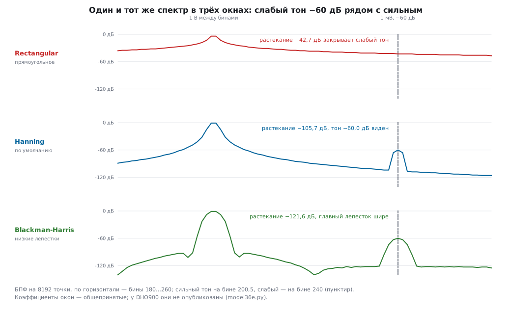
Why a window. The FFT treats the record as a piece of an endlessly repeating signal. If a non-integer number of periods fits into the record, there is a jump at the seam between repeats, and the energy of one frequency "leaks" into neighboring ones (leakage). A window smoothly brings the record edges to zero. The DHO900 has six: Rectangular, Blackman-Harris, Hanning (default), Hamming, Flattop and Triangle (User Guide p. 139; datasheet p. 17). The instrument's window coefficients are not published; the model uses the common definitions:
| window | noise bandwidth, bins | floor higher by | amplitude error between bins | side lobe | main lobe, bins |
|---|---|---|---|---|---|
| Rectangular | 1.00 | 0.00 dB | −3.92 dB | −13 dB | 1 |
| Triangle | 1.33 | 1.25 dB | −1.82 dB | −27 dB | 2 |
| Hamming | 1.36 | 1.34 dB | −1.75 dB | −43 dB | 2 |
| Hanning | 1.50 | 1.76 dB | −1.42 dB | −31 dB | 2 |
| Blackman-Harris | 2.00 | 3.02 dB | −0.83 dB | −92 dB | 4 |
| Flattop | 3.77 | 5.76 dB | −0.01 dB | −93 dB | 5 |
Every window buys something and pays for it: low side lobes cost a wide main lobe (close frequencies are harder to separate) and a larger noise bandwidth (a higher floor).
What you see — a weak line next to a strong one. A 1 V tone exactly between bins and a 1 mV tone (−60 dB) 40 bins away:
| window | leakage of the strong tone at the weak one | weak tone |
|---|---|---|
| Rectangular | −42.7 dB | not visible: −42.6 dB is the leakage |
| Hanning | −105.7 dB | visible: −60.0 dB |
| Blackman-Harris | −121.6 dB | visible: −60.0 dB |
Amplitude error. A tone between bins in the rectangular window is 3.92 dB below the true value — in voltage that is 0.64 of the true value. Flattop is off by 0.01 dB — that is why it is used for an accurate amplitude when the frequency does not fall on a bin.
Why the floor depends on the window. Each bin collects noise from its own band, and for a window that band is wider than one bin — by the amount in the "noise bandwidth" column. 1 mV of noise, 10 k points: the floor is −96.9 dBV in the rectangular window, −95.2 in Hanning, −94.0 in Blackman-Harris, −91.2 in Flattop. The noise itself is the same. And on the record length: with 1 M points the floor is −117.0 dBV — 20 dB lower, because a bin is 100 times narrower. Mistake: comparing the "noise level" of two spectra taken with different windows or different memory — they differ even on one and the same signal. Measure noise in the time domain (AC RMS, 36е.8).
Units. Unit: dBV, dBm or Vrms (User Guide p. 138). 0 dBV is 1 V RMS. A sine with an amplitude of 1 V is 0.7071 V RMS, −3.01 dBV. dBm is power relative to 1 mW in a load, usually 50 Ω: the same sine is +10.00 dBm. On a 1 MΩ input (the only one on the DHO900, 36г.6) dBm is a conversion convention; which load the instrument converts to, the User Guide does not say. Mistake: confusing amplitude and RMS — a 3 dB difference.
Which window when (from the User Guide table, p. 139, and the model): Hanning — the default, for periodic signals and noise; Blackman-Harris — weak harmonics next to a strong one; Flattop — accurate amplitude; Rectangular — a single pulse fully inside the record, or two close tones of equal strength; Hamming and Triangle — in between.
36е.23 FFT: square wave, PWM and aliasing
A 0/3.3 V square wave (model, integer number of periods): DC 1.650 V; the first harmonic has an amplitude of 2.101 V, RMS 1.486 V, +3.44 dBV; the third is 9.54 dB lower, the fifth 13.98 dB; there are no even ones at all. An even harmonic in the spectrum of a "square wave" is a sign that the duty cycle is not 50 % or the edges are asymmetric.
PWM. Harmonic number n is proportional to the sine of n·π·D divided by n, and becomes zero where n·D is an integer:
| harmonic relative to the first | 25 % | 10 % |
|---|---|---|
| 2nd | −3.01 dB | −0.44 dB |
| 3rd | −9.54 dB | −1.18 dB |
| 4th | none | −2.28 dB |
| 5th | −13.98 dB | −3.78 dB |
| 10th | −16.99 dB | none |
The DC part is 0.825 V at 25 % and 0.330 V at 10 %; the first harmonic is 1.050 V (+0.43 dBV) and 0.459 V (−6.76 dBV). A narrow pulse means an almost flat spectrum: the harmonics up to the tenth of a 10 % PWM are almost equal to the first. Case: LED PWM at 10 % and 20 kHz is heard in the audio path and seen in the ADC samples — its harmonics go far up almost without falling, and a filter for one frequency will not help.
Aliasing in the FFT. The instrument's front end passes hundreds of megahertz, while the sample rate on a slow time base is megahertz. Anything above half of it folds down (36г.15). Model: a 30 kHz square wave at 1 MSa/s (Nyquist limit 500 kHz). The 33rd harmonic at 990 kHz lands at 10 kHz — below the fundamental! — at −29.2 dB (its own level −30.4 dB); the 31st at 930 kHz gives a 70 kHz line at −28.8 dB (calculated −29.8). There are no 10 and 70 kHz lines in the signal. How to tell: change the time base — real lines stay, false ones move. Before an FFT, give the sample rate a margin: more memory or a faster time base, and look only at the lower part of the span.
36е.24 Bode plot (Bode Plot)
What it is. The built-in generator sweeps a sine in frequency, the instrument measures at each frequency the ratio of output to input (gain, dB) and the phase shift — and draws two curves (User Guide p. 194). Only on the DHO914S and DHO924S, which have the generator (same page); the generator itself is covered in 36к.
Settings (User Guide pp. 195–199; datasheet p. 19): In and Out — the input and output channels of the circuit; Sweep Type — Log or Line; FIR Setup — a digital filter; display — Wave (curves) or Chart (table of points). The start frequency is from 10 Hz to 24.99 MHz, the stop frequency from 100 Hz to 25 MHz; points from 10 to 300 — "per decade" by the User Guide and "per octave" by the datasheet; amplitude from 20 mV to 5 V or its own for frequency segments (Var.Amp.). The result is saved in CSV or HTML (p. 199).
What you see. An RC filter of 1 kΩ and 100 nF: at 1591.5 Hz the gain is −3.01 dB, the phase −45.0°. A sweep from 10 Hz to 100 kHz with 10 points per decade gives 41 points. After the sweep stops, the instrument shows the margins (User Guide p. 197): PM — how much phase is left to −180° at the frequency where the loop gain is 0 dB; GM — how far the gain is below 0 dB where the phase is −180°. The loop model is an integrator at 10 kHz and poles at 20 and 100 kHz: crossover 9.07 kHz, phase margin 60.4°, −180° at 44.7 kHz, gain margin 21.6 dB. What these margins mean — section 163.
How the loop is connected. The signal from the generator output goes through an isolation transformer to a resistor inserted into the feedback loop; the channels go on both sides of the resistor (User Guide p. 198).
Mistake. Too large an amplitude drives the loop out of its linear range, too small drowns in noise; the User Guide states directly that this function will not test noisy circuits (p. 195). Var.Amp. — a large amplitude where the loop strongly suppresses the signal and a small one where it amplifies.
Case. A regulator on the board (section 58) or a sensor amplifier: the phase margin with and without a capacitor at the output — two curves show why it rings with a small ceramic capacitor.
36е.25 Pitfalls
"No" overshoot. The Max-Min top method: Vtop = Vmax, overshoot 0.0 %, thresholds moved beyond the plateau (36е.7).
Duty cycle lower than set. A slow edge through a pull-up: 10 % in the firmware — 8.63 % at the middle threshold (36е.9).
An I2C edge "fails". Thresholds 10–90 % instead of 30–70 %: 4.13 µs instead of 1.59 µs (36е.10).
Frequency jumps on a slow signal. Noise at the threshold: 172 crossings per period (36е.9). BW Limit, a filter or the frequency counter.
Noise peak-to-peak differs on the same signal. Vpp grows with memory: 65 mV at 1 k points, 97 at 1 M (36е.6). Measure noise by AC RMS.
The mean jumps. A non-integer number of periods on the screen: +20 % on PWM (36е.8). Per.VRMS or more periods.
Power four times too low. The means were multiplied instead of taking the mean of the product (36е.17).
A−B on the 12 V rail. Channel errors of 120–172 mV with a signal of 50 mV (36е.17, 36з.5).
Wrong area. A zero offset of 1 mV over 10 ms adds +35.7 % to the charge of a burst (36е.13).
The derivative is all noise. 2.80 A of noise with a current of 0.50 A; smoothing (36е.18).
A weak harmonic is "missing". Rectangular window: leakage at −42.7 dB hides a −60 dB tone (36е.22).
A 10 kHz line on a 30 kHz square wave. Aliasing of the 33rd harmonic (36е.23).
Statistics without the rare event. 100 measurements miss a 0.2 % event with a probability of 81.9 % (36е.14).
The sixth digit of the frequency counter. The instrument's reference is ±25 ppm, at 8 MHz ±200 Hz (36е.16).
36е.26 Summary
- Cursors — when a person knows better than the instrument where the edge and the plateau are; automatic measurement — when the rule fits the signal. Indicator shows where the instrument took the number.
- Accuracy grows when the event is stretched across the screen: in time the error is a share of the screen width, in voltage a share of full scale.
- All automatic measurements rest on the top, the base and the 90/50/10 % thresholds. The top method (Histogram or Max-Min) and the thresholds change overshoot, edges, width, delay and phase. Set thresholds to the standard: I2C — 30–70 %.
- Vpp of noise grows with the record length, Vavg and VRMS are wrong on a non-integer number of periods; AC RMS and Per.VRMS are free of this.
- Statistics are for the maximum, the histogram for the shape of the distribution; the mean rarely answers "does it get worse".
- The frequency counter is only as accurate as the instrument's crystal (±25 ppm).
- Math: the mean of A×B is power, the product of the means is not; A−B does not measure a small difference on a large common mode; the derivative needs smoothing, the integral and the area need an accurate zero.
- FFT: the resolution is the reciprocal of the record duration; the window trades leakage, amplitude accuracy and floor height; the floor depends on the window and the number of points; above half the sample rate there is only aliasing.
- The Bode plot gives phase and gain margins if the sweep amplitude suits the circuit.
Next: section 36ж "Oscilloscope, part 4: bus decoding, masks, segmented memory, saving and SCPI control" — how the instrument reads UART, I2C, SPI and CAN, checks a signal against a mask (Pass/Fail), stores thousands of triggers, saves reference waveforms and how to control it from a computer.