 Embedded HandbookApps
56. Operational amplifiers
A sensor gives millivolts, the ADC expects volts. Between them sits an operational amplifier. Some microcontrollers already have one inside (section 44), but more often it is a separate chip, and then everything that was hidden you have to choose and calculate yourself.
This section is about how an op-amp is connected, what is non-ideal about it and which of the non-idealities will spoil your particular circuit.
Terms used in the documentation
Term Meaning operational amplifier (op-amp) a high-gain differential amplifier used with feedback negative feedback part of the output fed back to reduce the error inverting / non-inverting input the "−" / "+" input of the op-amp voltage follower, buffer unity-gain stage with high input impedance difference amplifier amplifies the difference of two voltages instrumentation amplifier difference amplifier with two high-impedance inputs input offset voltage (Vos) the parasitic voltage between the inputs input bias current (Ib) the current that flows into the inputs gain-bandwidth product (GBW) gain times bandwidth, constant for a given op-amp slew rate the maximum rate of change of the output common-mode rejection ratio (CMRR) how well a voltage common to both inputs is suppressed rail-to-rail input / output input / output range up to the supply rails single supply one supply voltage instead of ± virtual ground a node held at ground potential by feedback comparator compares two voltages, the output switches hysteresis different thresholds for rising and falling capacitive load a capacitance on the output isolation resistor a resistor that decouples the output from the load
56.1 Three configurations you need to know
Negative feedback forces the amplifier to keep the same voltage on both inputs. All the circuits follow from this one rule.
| Configuration | Gain | Input resistance |
|---|---|---|
| follower | ×1 | huge |
| non-inverting | 1 + Rос/Rз |
huge |
| inverting | −Rос/Rз |
equal to Rз |
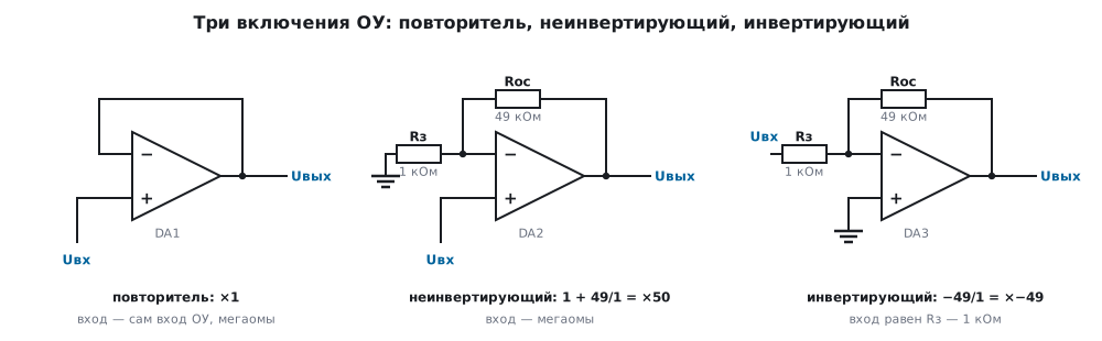
With 1 kΩ and 49 kΩ resistors the non-inverting stage gives ×50, and the inverting one on the same resistors gives ×49 (one less in magnitude; this is not a typo but a consequence of the circuit).
The main practical difference is not the sign but the input. For the inverting stage the input resistance equals the lower leg, 1 kΩ here. Connect to it a sensor with an internal resistance of 100 kΩ and you lose 99 % of the signal before any amplification. For the non-inverting stage and the follower the input is the input of the op-amp itself, megohms and more; the loss is less than one millionth.
An ngspice model (an op-amp with a gain-bandwidth product of 1 MHz) confirms this: from a 100 kΩ source the inverting ×49 gives at the output only 0.49 of the signal, the non-inverting one gives 49.9.
Hence the rule: a high-impedance source needs a non-inverting stage or a follower. The inverting stage is convenient when the source has low impedance, when you need a summing input or when a virtual ground matters (for example, for a photodiode).
56.2 Bandwidth: gain and frequency trade against each other
An op-amp is characterised by its gain-bandwidth product. If it equals 1 MHz:
| Gain | Bandwidth |
|---|---|
| ×1 | 1000 kHz |
| ×10 | 100 kHz |
| ×50 | 20 kHz |
| ×100 | 10 kHz |
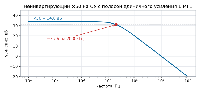
Our ×50 gives 20 kHz — but that is the −3 dB point, where the amplitude is already 29 % lower. The roll-off is gradual: at 10 kHz the signal loses 10.6 %, at 3 kHz — 1.1 %. For measurement, bandwidth is taken with margin: 7 times the signal frequency for 1 % accuracy and 22 times for 0.1 %. So for a current-sensor signal at 10 kHz with ×50 you need a part with a gain-bandwidth product of at least 3.5 MHz (1 %) or 11 MHz (0.1 %).
The model of the same ×50: 34.0 dB at low frequencies and −3 dB at 20.0 kHz, beyond that the gain falls by 20 dB per decade.
Separately — the slew rate. It limits not the small-signal bandwidth but the swing of a large signal. At 1 V/µs an output with a 3.3 V swing will not pass frequencies above 96 kHz, while for a 100 mV swing the same part handles 3.2 MHz. It covers the full swing in 3.3 µs.
On a follower model a 200 kHz sine with a 3.1 V swing comes out as a triangle with a 2.37 V swing: the slope is exactly 1.00 V/µs, the op-amp cannot go faster.
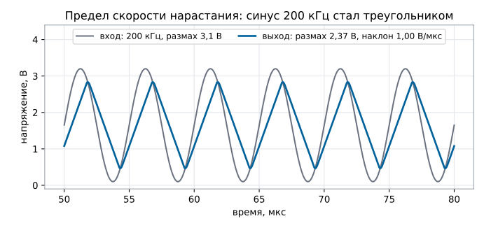
The smaller of the two limits applies, and you must not confuse them: "the bandwidth is enough, but the waveform is still triangular" — that is the slew rate.
56.3 Offset: the main error at high gain
In a real op-amp the inputs are not quite identical: between them there is a parasitic difference of a few millivolts. It is amplified together with the signal.
An offset of 3 mV at a gain of ×50 gives 150 mV at the output — 4.5 % of full scale, and that is with zero input signal.
What this means for current measurement with a shunt (the same task as in section 44.8):
| Value | |
|---|---|
| 10 mΩ shunt at 5 A | 50 mV of useful signal |
| offset of an ordinary op-amp, 3 mV | 6 % of the signal |
| reading at zero current | 0.3 A |
| offset of a precision part, 25 µV | 2.5 mA |
| drift 5 µV/°C over 60 degrees | another 30 mA |
The difference between an ordinary and a precision part is 120 times, and that is exactly what you pay for when you choose. Gain has nothing to do with it: by increasing it you increase the error too.
56.4 Input bias current: the error people forget
In an op-amp with a bipolar input a current flows into the inputs — about 100 nA. On the source resistance it turns into a voltage:
| Source resistance | Error |
|---|---|
| 1 kΩ | 0.1 mV |
| 100 kΩ | 10 mV |
| 1 MΩ | 100 mV |
With a high-impedance source this error is larger than the offset. In an op-amp with a FET input the bias current is about 1 pA — on the same megohm only 1 µV, a hundred thousand times less.
The rule: a source of hundreds of kilohms and above needs a FET input. A piezo sensor, a photodiode, an electrode, a high-impedance divider — all of them.
The error is partly compensated by making the resistances at both inputs equal: then equal currents give equal voltages, and the difference cancels. But the mismatch of the bias currents between the inputs remains.
56.5 The difference amplifier and the common-mode signal
The task of high-side current measurement: the shunt sits at 12 V, and you need to measure 50 mV across it. A difference amplifier on four resistors subtracts one from the other — in theory.
In practice its ability to reject the common-mode signal is entirely determined by the accuracy of the resistors:
| Resistor tolerance | Rejection | 12 V leaks through as |
|---|---|---|
| 5 % | 20 dB | 1.2 V |
| 1 % | 34 dB | 240 mV |
| 0.1 % | 54 dB | 24 mV |
| ready-made shunt amplifier, 90 dB | 90 dB | 379 µV |
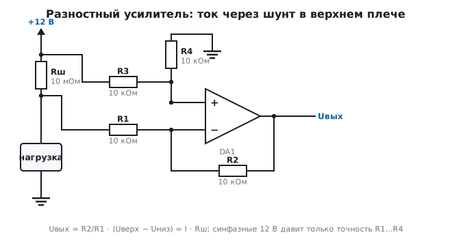
A model with the worst combination of 1 % resistors (two at +1 %, two at −1 %) with 12 V common-mode and zero difference gives 238 mV at the output — the estimate from the formula in the table is rounded to 240.
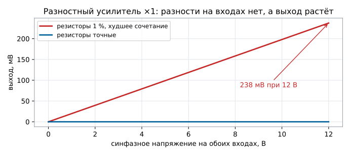
With ordinary 1 % resistors the error from 12 V common-mode (240 mV) is larger than the measured signal itself of 50 mV. Even 0.1 % resistors leave 24 mV — half the signal.
Also keep in mind the voltage on the op-amp inputs themselves: with four identical resistors they see half the common-mode voltage — 6 V. An op-amp supplied from 3.3 or 5 V cannot be connected like that. You need attenuating legs: R2/R1 = 1/5 gives 2 V at the inputs, but also attenuates the useful signal five times, and makes common-mode rejection even worse: with 1 % resistors — from 34 down to 29.5 dB. The error from 12 V at the output is 80 mV against a useful 10 mV, eight times larger than the signal.
The conclusion is harsh: a difference amplifier on discrete resistors is suitable where the common-mode voltage is small. For high-side current measurement you take a dedicated shunt amplifier: its input is rated for common-mode voltages up to tens of volts with a 3.3 V supply, and its resistors are laser-trimmed right on the die. An ordinary instrumentation amplifier will not help here: its inputs must stay within its own supply range (section 176).
An instrumentation amplifier also differs from a difference amplifier in its input: it has both inputs high-impedance (three op-amps inside), so it does not load the source, and the gain is set by a single external resistor.
56.6 Single supply
Classic circuits are drawn with two supplies, ±15 V. On a board with a microcontroller there is one supply: 3.3 or 5 V. This leads to two peculiarities.
Mid-scale. An AC signal (for example, audio or a current of alternating polarity) is shifted to the middle — 1.65 V with a 3.3 V supply, which is code 2048 for a 12-bit ADC. But the bias is applied only through DC isolation: if you apply 1.65 V to the input of an amplifier with ×50, the output would be 82.5 V — the output immediately hits the supply rail.
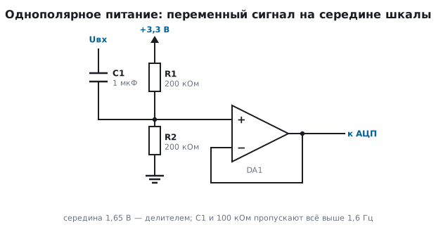
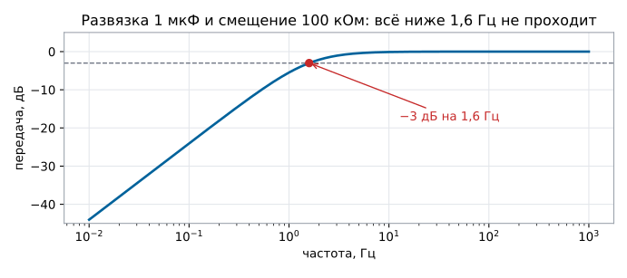
The coupling capacitor sets the lower edge of the bandwidth: 1 µF and a 100 kΩ bias divider give a cut-off of 1.6 Hz. Fine for audio; for a slow sensor it is not: such a circuit will not pass the DC component at all. Slow signals are amplified without coupling, and the bias is introduced differently — through the second input of a difference circuit.
The model of this circuit: exactly 1.65 V at the output, the −3 dB edge is at 1.59 Hz.
Output swing. An ordinary op-amp does not reach the supply rails by roughly 1.5 V on each side: at 3.3 V that leaves 0.3 V of useful swing, so the part is useless. You need a rail-to-rail one — it keeps 3.2 V out of 3.3. The same goes for the input: if the signal comes from ground level, the input must also be rail-to-rail.
56.7 Comparator with hysteresis and capacitive load
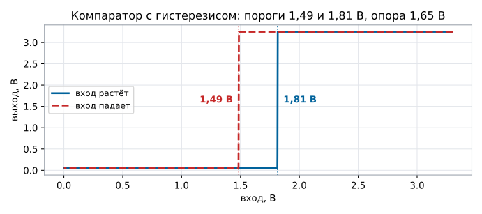
Comparator. Without feedback an op-amp turns into a comparator: the output hits one of the supply rails depending on which input is higher. A noisy signal near the threshold will make it chatter dozens of times. The cure is positive feedback: through R2 the output pushes the non-inverting input and shifts the threshold.
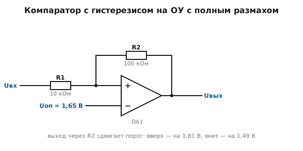
The rising threshold is Uоп · (1 + R1/R2) − Uвых.низ · R1/R2, the falling threshold is the same
with Uвых.верх. With a 1.65 V reference, R1 = 10 kΩ, R2 = 100 kΩ and an output
that stays 0.05 V short of the rails, you get 1.81 V rising and 1.49 V
falling — a hysteresis of 0.32 V (output swing 3.2 V × R1/R2). The model switches
at almost the same points — at 1.815 and 1.485 V, hysteresis 0.33 V:
A dedicated comparator chip switches faster and does not mind staying in saturation for long, but for slow signals — a temperature threshold, battery monitoring — a rail-to-rail op-amp is enough.
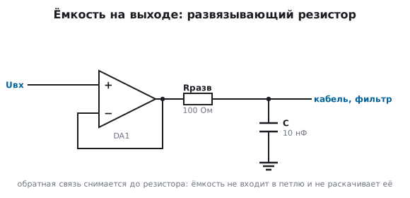
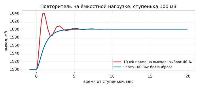
Capacitive load. The output resistance of the op-amp together with the capacitance of a cable or a filter adds one more delay to the loop, and the follower starts to ring. The cure is a resistor of tens of ohms between the output and the capacitance, with the feedback taken before it.
A model of a follower with an output resistance of 50 Ω into 10 nF: a 100 mV step gives 40 % overshoot and decaying ringing; with a 100 Ω resistor there is no overshoot.
56.8 How to choose
| What matters | What to look at |
|---|---|
| high-impedance source | FET input, low bias current |
| millivolt signal | low offset and its drift |
| fast signal | gain-bandwidth product and slew rate |
| single 3.3 V supply | rail-to-rail input and output |
| measurement at high common-mode voltage | a shunt amplifier with the required common-mode range |
| battery-powered device | quiescent current (from 1 µA to 10 mA) |
| ADC after the op-amp | input-referred noise |
And a general tip: if the microcontroller has a built-in op-amp (section 44), first check whether it is enough. It is not a precision part, but it is free, already matched to the ADC and takes no board space.
56.9 Pitfalls
The sensor signal dropped several times. An inverting stage loaded a high-impedance source.
There is voltage at the output with zero input. Offset multiplied by gain. Either take a precision part or subtract the zero in software (measuring it at a known zero signal).
The readings drift as the board warms up. Offset drift.
The error grows with the sensor resistance. Bias current of a bipolar input.
The difference amplifier "sees" the common-mode voltage. Resistor accuracy; 1 % gives only 34 dB.
The output does not reach the required level. The part is not rail-to-rail, or the load resistance is too low.
The waveform became triangular. You hit the slew rate, not the bandwidth.
The circuit oscillates. A capacitive load on the output (a long cable, a filter capacitor) — you need a resistor of tens of ohms between the output and the load (56.7).
The comparator chatters on a slow signal. No hysteresis: add positive feedback.
Amplified a thousand times, got noise. Offset, drift and noise are amplified together with the signal; at high gains the signal is filtered first, and the gain is split between two stages.
56.10 Summary
- Feedback keeps the inputs equal — all configurations follow from this.
- The inverting stage loads the source with the resistance of the lower leg: a 100 kΩ source loses 99 % of the signal.
- Gain-bandwidth product: ×50 from a 1 MHz part gives 20 kHz at −3 dB, and at 10 kHz the signal is already 10.6 % lower; separately there is the slew-rate limit — 96 kHz for a 3.3 V swing at 1 V/µs.
- An offset of 3 mV at ×50 is 150 mV at the output and 0.3 A of apparent current on a 10 mΩ shunt; a precision part gives 2.5 mA.
- A bias current of 100 nA on a 1 MΩ source is 100 mV of error; a FET input gives 1 µV.
- Common-mode rejection of a difference amplifier is set by the resistor tolerance: 1 % gives only 34 dB, and 12 V turns into 240 mV of error.
- A single supply requires a rail-to-rail part and careful injection of the mid-scale; 1 µF coupling with 100 kΩ cuts everything below 1.6 Hz.
- A comparator with a 1.65 V reference, 10 kΩ at the input and 100 kΩ of feedback switches at 1.81 V rising and 1.49 V falling; 10 nF directly on the follower output gives 40 % overshoot, a 100 Ω isolation resistor removes it.
Next: section 57 "PWM in power electronics" — what happens when the switches from section 52 start switching fast and with a purpose.