 Embedded HandbookApps
121. Classic versus ML: the Kalman filter and battery state of charge
You cannot measure a battery's state of charge — you can only estimate it from current and voltage. The task looks made for a neural network: there are inputs, there is an answer, and the test bench gives as much data as you want. This section sets up a fair comparison: coulomb counting, a voltage lookup table, an extended Kalman filter on a physical battery model, and a neural network trained on thousands of seconds of discharge — on a familiar load, on an unfamiliar one and on an aged battery. The conclusion of part XIV: when the physics is known, its model with feedback from the measurement beats a trained one — especially where the world has moved away from the training data.
The experiments run in the stm-ml:1 image; the C filter is checked against Python and built
for F407 and F103. The Kalman filter is introduced here from scratch; models and their
training are in sections 116–118.
What it is called in the documentation
Original Meaning state of charge (SoC) charge as a fraction of full capacity coulomb counting integrating the current open-circuit voltage (OCV) voltage with no load equivalent circuit model the battery's equivalent circuit extended Kalman filter (EKF) Kalman filter for nonlinear models state, covariance the state and its covariance process / measurement noise noise of the process / of the measurement innovation residual: measurement minus prediction Jacobian matrix of derivatives observability whether the state can be seen from the measurements sensor offset (bias) sensor zero offset state of health, ageing battery health, ageing joint (augmented) estimation estimating the state and a parameter together battery management system (BMS) battery management system
121.1 The battery as a circuit
The equivalent circuit of a lithium cell: an open-circuit voltage source that depends on the charge (a table of 11 points from 3.00 to 4.20 V), a series resistance R0 = 0.05 Ω and an RC network R1 = 0.03 Ω, C1 = 1000 F — the slow part of the voltage sag, with a time constant of 30 s. Capacity 2.5 A·h. Step 1 s. The current sensor has a constant error of 0.05 A and noise of 0.02 A, the voltage sensor has 5 mV of noise — typical figures for a shunt with an amplifier and a 12-bit ADC.
The model is for an ordinary 4.2 V cell at room temperature. In the cold R0 grows several times, so a product takes the parameters from a table by temperature. For LiFePO4 the voltage in the middle of the charge range barely changes (3.2–3.3 V): the slope is small, and there the filter relies mostly on coulomb counting — only the ends of the scale give a correction.
Three test loads: the same kind as when training the neural network (bursts of 0.5–3 A of different length); a different one — a steady 1.2 A with short bursts up to 4 A; the same different one, but on an aged battery — capacity 12 % lower, R0 1.6 times higher. All estimators except coulomb counting start from a charge of 0.5 while the true one is 0.9: the device restarted under load and does not know the initial charge.
121.2 Coulomb counting and the table
Coulomb counting adds up the current: the charge drops by I·Δt / Q every step. It is smooth and accurate over a short stretch, but it accumulates everything: an offset of 0.05 A over an hour and a half is 3 % of charge, and a wrong capacity on an old battery adds more. And it needs the initial charge — here it was given exactly.
The voltage table is the inverse problem: the charge at which the open-circuit voltage equals the measured one. Under load the measured voltage has sagged by I·R0 and by the RC network, and the error reaches tens of percent. The table is right only after a long rest — and that is how it is used: for the initial charge after a night.
121.3 The extended Kalman filter
The Kalman filter combines both methods: a prediction from the current, like coulomb counting, and a correction from the voltage, like the table — with a weight that it computes itself from how much it trusts the prediction and the measurement. The state is the charge and the RC network voltage; the terminal voltage depends on the charge nonlinearly, so the filter is extended: the correction uses the slope of the table at the current point.
A filter step in C — the prediction:
e->x[0] -= i * DT_Q;
e->x[1] = A_RC * e->x[1] + R1 * (1.0f - A_RC) * i;
The correction by the innovation — the difference between the measured and predicted voltage:
yhat = ocv(e->x[0], &slope) - e->x[1] - e->x[2] * i;
S = H[0] * PH[0] + H[1] * PH[1] + H[2] * PH[2] + R_V;
y = v - yhat;
K[r] = PH[r] / S;
e->x[r] += K[r] * y;
The code is taken from the filter that runs on the device (121.8), and its state
already has three numbers: the third, x[2], is the resistance R0 (121.5). In
a simple two-state filter, e->x[2] is replaced by the constant
R0 = 0.05 Ω, and H, PH and K have two elements.
Besides the estimate, the filter keeps the covariance P — how sure it is of the estimate.
The prediction grows it, P = F·P·Fᵀ + Q; the transition matrix F is diagonal —
1, A_RC, 1 — so two loops are enough:
for (r = 0; r < 3; r++)
    for (c = 0; c < 3; c++)
        e->P[r][c] *= F[r] * F[c];
for (r = 0; r < 3; r++)
    e->P[r][r] += QD[r];
H is the sensitivity of the terminal voltage to each state: to the charge —
the table slope, to the RC network voltage — −1, to R0 — −i; PH = P·Hᵀ:
H[0] = slope;
H[1] = -1.0f;
H[2] = -i;
for (r = 0; r < 3; r++)
    PH[r] = e->P[r][0] * H[0] + e->P[r][1] * H[1] + e->P[r][2] * H[2];
After the correction the covariance shrinks, P = (I − K·H)·P:
for (r = 0; r < 3; r++)                 /* P = (I − K·H)·P, P симметрична: H·P = PHᵀ */
    for (c = 0; c < 3; c++)
        e->P[r][c] -= K[r] * PH[c];
Two settings decide everything: Q — how much the filter distrusts the prediction,
R_V — how much it distrusts the measurement. In the experiment the diagonal of Q is 10⁻⁷
for the charge, 10⁻⁶ V² for the RC network and 10⁻¹⁰ Ω² for R0, and R_V = 10⁻⁴ V²,
that is (10 mV)²: twice the 5 mV noise of the voltage sensor, with a margin for
model inaccuracy. A larger Q makes the filter more willing to believe the voltage, a larger
R_V makes it hold on harder to coulomb counting.
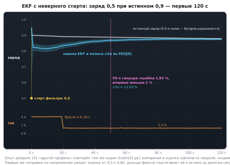
From the wrong start of 0.5 the filter converged to the true charge within 2 % in 50 seconds: a few current bursts — and the voltage revealed where the battery really is.
121.4 Sensor offset in the state — and observability
A current offset accumulates error in coulomb counting; the natural idea is to add it to the filter state and let the filter estimate it. The result is the opposite of what you expect: on a new battery the filter with the offset is worse than the simple one, and the offset itself was estimated as 0.085 A instead of 0.05. The current offset is poorly observable: its trace in the voltage is an I·R0 error of 2.5 mV, less than the sensor noise, and in the charge it cannot be told apart from a slightly different capacity. The simple filter copes with the offset anyway: the voltage correction does not let the error accumulate. An extra state that the measurements cannot see only adds noise.
121.5 R0 in the state: the filter tracks ageing
Ageing changes two parameters at once: capacity and resistance. A filter with the datasheet R0 and capacity explains the extra voltage sag of an old battery by a lower charge — and is off by 5–10 %. The resistance, however, is very well observable: every current burst shows it directly, as a voltage step. The third state is R0, slowly drifting:
x = np.array([s0, 0.0, R0])
H = np.array([docv(x[0]), -1.0, -i])
The filter estimated R0 of the old battery as 0.0787 Ω with a true value of 0.08 — and the charge error dropped to one percent. Capacity can be added to the state in the same way, but it is visible only over a whole discharge cycle; in industrial systems it is adjusted separately, over full cycles.
121.6 The neural network
The neural network gets the same inputs as the filter: voltage and current, plus their averages over a minute — to see the slow part of the sag. Two hidden layers of 16 neurons, 369 weights, 48252 training samples from 12 discharges from different initial charges with the same equivalent circuit. It has one advantage, but an important one: it does not accumulate state and does not need the initial charge — the answer comes from the last minute.
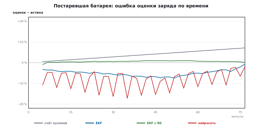
On the familiar load it is a little worse than the filter, on the unfamiliar one almost the same. It has never seen an old battery: for it a sag 1.6 times larger simply means a lower charge, and the error reaches one fifth. It can be retrained only on data from old batteries, which do not yet exist when the device is released.
121.7 Comparison
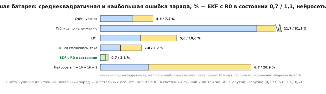
RMS / maximum charge error, %, after the first 10 minutes:
| Method | Same load | Different load | Aged battery |
|---|---|---|---|
| Coulomb counting | 1.8 / 3.0 | 1.8 / 3.0 | 4.5 / 7.3 |
| Voltage table | 17.3 / 37.9 | 16.6 / 48.4 | 21.7 / 61.3 |
| EKF | 0.5 / 0.9 | 0.6 / 0.9 | 5.6 / 10.6 |
| EKF with current offset | 1.1 / 1.8 | 0.9 / 1.5 | 2.8 / 5.7 |
| EKF with R0 in the state | 0.2 / 0.5 | 0.3 / 0.7 | 0.7 / 1.1 |
| Neural network 4 → 16 → 16 → 1 | 0.9 / 3.4 | 1.0 / 4.0 | 6.7 / 20.9 |
Coulomb counting was given the exact initial charge — the others do not have it. The filter with R0 in the state is the best in all three cases. The neural network loses to the simple filter and to the filter with R0 everywhere, and on the old battery its error is larger than even coulomb counting.
121.8 On the device
The C filter is 12 float numbers: three state numbers and a 3 × 3 matrix, the state is 48 bytes; the voltage table is 44 bytes. armclang: 558 bytes of code on F407 and 908 on F103, where float is done in software. A run over 4700 seconds of the old battery matched numpy to a millionth. One step per second is a few hundred floating-point operations; on F103 without an FPU that is a fraction of a millisecond.
The neural network has 369 weights — 1476 bytes in float, in int8 as in section 119 about half a kilobyte. It does not come out smaller than the filter, and it has to be computed once a second just the same.
Practice in battery management systems: the filter is the core, the table gives the initial charge after rest, coulomb counting sits inside the filter as the prediction. Where a neural network is used, it stands beside the filter — for example, it estimates a parameter that the physical model does not describe (dependence on temperature, ageing from history) — and passes it to the filter.
121.9 What to choose when
- The physics is known and measured directly — a model and a Kalman filter. It is explainable: you can see which state changed and why.
- The physics is known, the parameters drift — a filter with the parameter in the state, if the parameter is observable; check this by experiment, as with the current offset.
- There is no physics or it is too complex (vibration, sound, images) — training, sections 116–120.
- There is no training data for future conditions (ageing, a new cell supplier) — do not rely on a single trained model.
121.10 Pitfalls
The filter converges to the wrong charge. Wrong model parameters: the filter blames the sag from ageing on the charge. Put the resistance in the state, adjust the capacity over full cycles.
We added a state and it got worse. The state is poorly observable: the current offset was estimated as 0.085 A instead of 0.05. Check whether the measurement sees it, and do not add anything extra.
The filter diverged after a day of operation. The matrix P lost symmetry or positive definiteness due to float rounding. Symmetrize P, clamp the diagonal from below, use the Joseph form for the update.
Coulomb counting drifted by a few percent. Zero offset of the current sensor. Calibrate the zero at zero current, correct from the voltage after rest.
The neural network confidently lies on a new battery. Conditions outside the training data. Before release, test on conditions that were not in the training.
121.11 Summary
- The voltage table under load is off by tens of percent, coulomb counting accumulates the offset and the capacity error.
- The EKF combines the prediction from current and the correction from voltage: from a wrong start it converged in 50 seconds, error 0.5 %.
- R0 in the state: the filter estimated 0.0787 Ω with a true value of 0.08 and on the old battery holds 0.7 % against 5.6 % without it.
- Neural network: 1.0 % on an unfamiliar load, 6.7 % and up to 20.9 % on the old battery — outside the training data.
- Filter: 558 bytes of code on F407, state — 48 bytes.
Part XIV is complete: from choosing the approach (116) and the features (117) through training (118), quantization (119) and models of normal behaviour (120) to the boundary where a trained model gives way to a physical one.
Full sources
ekf121.c — extended Kalman filter for battery charge with the state [charge, U_RC, R0].
/* Раздел 121: расширенный фильтр Калмана заряда батареи — состояние [заряд, U_RC, R0].
 * С -DML_HOST main() прогоняет измерения постаревшей батареи и сверяет с numpy. */
#include "model121.h"

typedef struct {
    float x[3];                 /* заряд 0…1, напряжение RC-цепочки, В, сопротивление R0, Ом */
    float P[3][3];
} ekf_t;

static const float QD[3] = { 1e-7f, 1e-6f, 1e-10f };

/* Напряжение холостого хода и его наклон по таблице из 11 точек через 0,1. */
static float ocv(float s, float *slope)
{
    int k = (int)(s * 10.0f);
    float t;
    if (k < 0)
        k = 0;
    if (k > N_PTS - 2)
        k = N_PTS - 2;
    *slope = (OCV_T[k + 1] - OCV_T[k]) * 10.0f;
    t = s * 10.0f - (float)k;
    if (s <= 0.0f)
        return OCV_T[0];
    if (s >= 1.0f)
        return OCV_T[N_PTS - 1];
    return OCV_T[k] + (OCV_T[k + 1] - OCV_T[k]) * t;
}

void ekf_init(ekf_t *e, float soc0)
{
    int i, j;
    for (i = 0; i < 3; i++)
        for (j = 0; j < 3; j++)
            e->P[i][j] = 0.0f;
    e->x[0] = soc0;
    e->x[1] = 0.0f;
    e->x[2] = R0;
    e->P[0][0] = 0.1f;
    e->P[1][1] = 0.01f;
    e->P[2][2] = 1e-4f;
}

/* Один шаг 1 с: прогноз по току, коррекция по напряжению. */
void ekf_step(ekf_t *e, float v, float i)
{
    float F[3] = { 1.0f, A_RC, 1.0f };     /* матрица перехода диагональна */
    float H[3], PH[3], S, K[3], y, slope, yhat;
    int r, c;

    e->x[0] -= i * DT_Q;
    e->x[1] = A_RC * e->x[1] + R1 * (1.0f - A_RC) * i;
    for (r = 0; r < 3; r++)
        for (c = 0; c < 3; c++)
            e->P[r][c] *= F[r] * F[c];
    for (r = 0; r < 3; r++)
        e->P[r][r] += QD[r];

    yhat = ocv(e->x[0], &slope) - e->x[1] - e->x[2] * i;
    H[0] = slope;
    H[1] = -1.0f;
    H[2] = -i;
    for (r = 0; r < 3; r++)
        PH[r] = e->P[r][0] * H[0] + e->P[r][1] * H[1] + e->P[r][2] * H[2];
    S = H[0] * PH[0] + H[1] * PH[1] + H[2] * PH[2] + R_V;
    y = v - yhat;
    for (r = 0; r < 3; r++) {
        K[r] = PH[r] / S;
        e->x[r] += K[r] * y;
    }
    for (r = 0; r < 3; r++)                 /* P = (I − K·H)·P, P симметрична: H·P = PHᵀ */
        for (c = 0; c < 3; c++)
            e->P[r][c] -= K[r] * PH[c];
}

#ifdef ML_HOST
#include <math.h>
#include <stdio.h>
int main(void)
{
    ekf_t e;
    int n;
    float worst = 0.0f, worst_r = 0.0f;
    ekf_init(&e, S0);
    for (n = 0; n < N_SAMPLES; n++) {
        ekf_step(&e, MEAS_V[n], MEAS_I[n]);
        if (fabsf(e.x[0] - REF_SOC[n]) > worst)
            worst = fabsf(e.x[0] - REF_SOC[n]);
        if (fabsf(e.x[2] - REF_R0[n]) > worst_r)
            worst_r = fabsf(e.x[2] - REF_R0[n]);
    }
    printf("steps=%d\nworst_soc_ppm=%d\nworst_r0_uohm=%d\nsoc_end=%.4f\nr0_end=%.4f\n", N_SAMPLES,
           (int)(worst * 1e6f + 0.5f), (int)(worst_r * 1e6f + 0.5f), e.x[0], e.x[2]);
    return 0;
}
#else
volatile float g_v, g_i, g_soc;
void SystemInit(void) {}
int main(void)
{
    ekf_t e;
    ekf_init(&e, S0);
    for (;;) {
        ekf_step(&e, g_v, g_i);
        g_soc = e.x[0];
    }
}
#endif
Next: section 121а "OpenMV: a machine-vision camera on STM32H7 — DCMI, MicroPython and object search" — an open camera on the STM32H743: the frame through DCMI and MDMA, LAB thresholds and blob search with find_blobs, neural networks through TensorFlow Lite Micro.