 Embedded HandbookApps
120. Anomaly detection: vibration and predictive maintenance
Sections 116–119 taught a model to tell known states apart: normal operation, imbalance, a bearing fault. In a factory this is rarely possible: there are almost no recordings with defects, and the defect that does happen may turn out to be an unfamiliar one. It is more honest to ask a different question — "does this look like normal?" — and train the model on healthy operation only. This section compares four such methods on a shared model of normal operation and one on each device's own normal, learned right after installation, and shows why the second approach wins here by a huge margin.
The data comes from the generator of section 118, the features from section 117, and the experiments
run in the stm-ml:1 image.
Terms used in the documentation
Term Meaning anomaly (novelty) detection finding windows unlike anything seen before one-class learning training on one class only — normal operation predictive maintenance servicing a machine by its condition anomaly score a number for how unusual a window is z-score the deviation measured in units of spread Mahalanobis distance a distance that accounts for how features are related k-means normal operation described as several centres autoencoder, reconstruction error a network that rebuilds its input, and the error of that rebuild baseline the device's own normal Welford's algorithm mean and spread updated on the fly false alarm rate the share of false alarms detection rate the share of defects found threshold, percentile the decision level and how it is chosen concept drift normal operation changing over time
120.1 Normal operation instead of classes
A model of normal operation does not answer with the name of a defect but with a number — an anomaly score: the further a window is from everything the model has seen, the larger it is. The decision is a comparison with a threshold. The threshold is chosen on healthy windows: for example, so that 1 % of them end up above it. That is the expected false alarm rate; anything above the threshold on a working device is a reason to take a look at the motor.
The experiment is set up like the life of a device. The normal model is trained on 1200 windows from 30 healthy motors. The test is 60 devices, each on its own motor: for the first 20 windows the motor is healthy, then 20 devices develop an imbalance, 20 a bearing defect, and 20 keep running healthy. In total there are 400 windows with imbalance, 400 with the bearing fault and 1200 healthy ones.
120.2 z-score
The simplest method: for each feature, the mean and spread over normal operation; the score is the sum of squared deviations measured in units of spread. The four features of section 117 give eight model numbers. The method assumes the features are independent and bell-shaped; for vibration this is only partly true, but as a first line it works everywhere.
120.3 Mahalanobis, k-means, autoencoder
The Mahalanobis distance accounts for how features are related: on a healthy motor the RMS and the crest factor change together, and a window where they diverge is more suspicious than the sum of the separate deviations. The model is the mean and the inverse covariance matrix, 4 + 16 numbers.
k-means describes normal operation with several centres — useful when a healthy motor has several modes (idle, under load). The score is the squared distance to the nearest centre.
An autoencoder is a neural network that learns to reconstruct its input through a narrow bottleneck. Here the input is the whole spectrum, 64 bins, the bottleneck is 8 neurons, 1096 parameters:
ae = MLPRegressor(hidden_layer_sizes=(8,), max_iter=3000, random_state=120).fit((XS - smu) / ssd, (XS - smu) / ssd)
It reconstructs normal spectra well and unfamiliar ones badly; the score is the mean squared reconstruction error.
120.4 The device's own normal
The main obstacle from section 118 is that every motor has its own vibration strength, and every mounting its own sensitivity. A shared normal model has to treat all this variety as normal, and the imbalance of one motor ends up inside the normal range of another. The way out: let each device learn the normal of its own motor by itself — the first 10 windows (2.5 seconds) after installation, while the motor is healthy:
m, s = F[:10].mean(axis=0), F[:10].std(axis=0) + 1e-6
return (((F[10:] - m) / s) ** 2).sum(axis=1)
It is the same z-score, only the mean and spread are the device's own. The threshold is still chosen once for all devices — on the healthy windows of the training motors, each with its own baseline.
120.5 Results
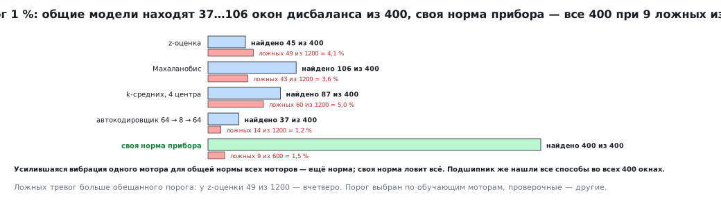
False alarms on healthy windows / imbalance windows found out of 400:
| Method | z-score | Mahalanobis | k-means, 4 centres | autoencoder 64 → 8 → 64 | own normal |
|---|---|---|---|---|---|
| Threshold 5 % | 67 / 106 | 85 / 140 | 138 / 113 | 66 / 74 | 49 / 400 |
| Threshold 1 % | 49 / 45 | 43 / 106 | 60 / 87 | 14 / 37 | 9 / 400 |
| Threshold 0.1 % | 31 / 40 | 16 / 40 | 26 / 40 | 0 / 8 | 3 / 400 |
False alarms are counted out of 1200 healthy windows for the shared models and out of 600 for the own normal (the first 10 windows of each device went into the baseline).
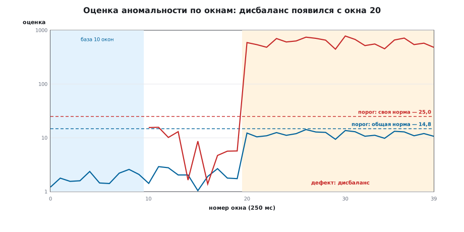
The bearing fault was found in all 400 windows by every method at every threshold: a new frequency in the spectrum gives itself away. The hard case is imbalance, that is, the same spectrum, only stronger. The shared models find from 8 to 140 windows out of 400: the increased vibration of one motor still fits within the normal range of all motors. The own normal finds all 400 at any threshold. The figure shows one such device: after the imbalance appeared, the shared model's score rose to 9–14 and did not reach the threshold, while the own normal's score rose to hundreds (threshold 25.0 versus 14.8 for the shared model).
One more thing: the shared models give more false alarms than the threshold promised — for the z-score at the 1 % threshold this is 49 windows out of 1200, four times more. The threshold was chosen on the training motors, and the test motors are different ones. The own normal is closer to the promise here as well: 9 out of 600.
120.6 The own normal on the device: Welford's algorithm
You do not need to store 10 windows to compute the mean and spread later: Welford's algorithm updates them one window at a time, without the loss of precision that the formula "mean of squares minus square of the mean" suffers from:
void base_add(baseline_t *b, const float f[N_FEAT])
{
    int i;
    b->n++;
    for (i = 0; i < N_FEAT; i++) {
        float d = f[i] - b->mean[i];
        b->mean[i] += d / (float)b->n;
        b->m2[i] += d * (f[i] - b->mean[i]);
    }
}
The score of a window is the same sum of squares:
float sd = sqrtf(b->m2[i] / (float)b->n) + 1e-6f;
float z = (f[i] - b->mean[i]) / sd;
s += z * z;
A run on the windows of two devices: the alarms from C and numpy matched in all 60 windows, and the scores differ by tens of parts per million — float versus double. armclang: the three functions take 390 bytes on the F407 and 512 on the F103 (no FPU, not counting the floating-point library); the state is 36 bytes: a counter, four means and four sums.
120.7 When to learn the normal
The baseline is learned after installation and after every repair — on a command from the technician, not on its own. If the device is installed on a motor that is already faulty, it will learn the fault as normal; the safeguard against this is the shared model, which runs alongside and catches what stands out strongly on all motors (the bearing fault in the experiment). Two levels — shared and own — are the usual scheme in industrial systems.
Normal operation changes slowly: wear, temperature, season. If the baseline is pulled towards new windows, the device will also get used to a slowly growing defect. So the baseline is not updated on the fly; it is relearned on command, and the history of scores is kept: a smooth rise of the score over weeks is the most valuable signal in predictive maintenance.
120.8 Threshold and alarm
A percentile threshold is only the beginning. On a device the alarm is raised not on a single window but on several in a row: with 1 % false positives per window and the rule "3 windows out of 5", a false alarm happens roughly a thousand times less often (if the windows are independent), while a real defect persists in every window and passes the rule with a delay of only three windows — as many anomalous windows as the rule needs. Besides the alarm, it is useful to report the score itself upstream: it shows how far the motor has drifted, not just "yes or no".
120.9 Which method to choose
- Own normal on a z-score — the first choice if the device sits on one motor: 36 bytes, no training on a computer, the best result.
- Mahalanobis — when the features are noticeably related; 20 numbers, the same arithmetic.
- k-means — when normal operation has several operating modes.
- Autoencoder — when there are no features and you have to work with the spectrum; a thousand parameters, quantized as in section 119.
120.10 Pitfalls
The device learned a defect as normal. The baseline was taken on a motor that was already faulty. Learn the baseline after repair and keep a shared model alongside.
More false alarms than the threshold promised. The threshold was chosen on other motors. Use the device's own normal or a threshold from the device's first hours of operation.
An alarm from a single window. A knock, a transient, a start-up. Use the rule "several windows in a row".
The device got used to a growing defect. The baseline is pulled towards new windows. Relearn only on command and keep the history of scores.
A feature's spread is almost zero — the score shoots up. The feature did not change in the baseline. Use a minimum spread (here 1e−6) or a lower bound based on the sensor noise.
120.11 Summary
- A normal model answers with a score; the decision is a threshold chosen on healthy windows.
- A new frequency (bearing fault) is visible to any method: 400 out of 400.
- A stronger version of the same vibration (imbalance) is almost invisible to the shared normal — from 8 to 140 out of 400; the device's own normal finds 400 out of 400.
- The own normal is Welford's algorithm: 36 bytes of state, 390 bytes of code on the F407.
- The baseline is learned on command after installation and repair; the most valuable signal is a smooth rise of the score over weeks.
Full sources
anom120.c — the device's own normal: mean and spread by Welford's algorithm and a z-score for each window.
/* Раздел 120: своя норма прибора — среднее и разброс признаков по алгоритму Уэлфорда,
 * затем z-оценка каждого окна. С -DML_HOST main() сверяет оценки и тревоги с numpy. */
#include <math.h>
#include "model120.h"

typedef struct {
    unsigned n;
    float mean[N_FEAT], m2[N_FEAT];
} baseline_t;

void base_reset(baseline_t *b)
{
    int i;
    b->n = 0;
    for (i = 0; i < N_FEAT; i++)
        b->mean[i] = b->m2[i] = 0.0f;
}

/* Одно окно нормы: среднее и сумма квадратов отклонений обновляются без хранения окон. */
void base_add(baseline_t *b, const float f[N_FEAT])
{
    int i;
    b->n++;
    for (i = 0; i < N_FEAT; i++) {
        float d = f[i] - b->mean[i];
        b->mean[i] += d / (float)b->n;
        b->m2[i] += d * (f[i] - b->mean[i]);
    }
}

/* Оценка окна: сумма квадратов отклонений в долях разброса нормы. */
float base_score(const baseline_t *b, const float f[N_FEAT])
{
    float s = 0.0f;
    int i;
    for (i = 0; i < N_FEAT; i++) {
        float sd = sqrtf(b->m2[i] / (float)b->n) + 1e-6f;
        float z = (f[i] - b->mean[i]) / sd;
        s += z * z;
    }
    return s;
}

#ifdef ML_HOST
#include <stdio.h>
int main(void)
{
    int d, w, k = 0, alarms_same = 0, n = 0, alarms = 0;
    float worst = 0.0f;
    for (d = 0; d < N_DEV; d++) {
        baseline_t b;
        base_reset(&b);
        for (w = 0; w < N_BASE; w++)
            base_add(&b, &WIN[(d * N_WIN + w) * N_FEAT]);
        for (w = N_BASE; w < N_WIN; w++, k++) {
            float s = base_score(&b, &WIN[(d * N_WIN + w) * N_FEAT]);
            float rel = fabsf(s - REF[k]) / (REF[k] + 1.0f);
            if (rel > worst)
                worst = rel;
            alarms_same += (s > THRESH) == (REF[k] > THRESH);
            alarms += s > THRESH;
            n++;
        }
    }
    printf("alarms_same=%d,%d\nalarms=%d\nworst_ppm=%d\n", alarms_same, n, alarms, (int)(worst * 1e6f + 0.5f));
    return 0;
}
#else
volatile float g_feat[N_FEAT];
volatile int g_alarm;
void SystemInit(void) {}
int main(void)
{
    baseline_t b;
    float f[N_FEAT];
    int i, w;
    base_reset(&b);
    for (w = 0;; w++) {
        for (i = 0; i < N_FEAT; i++)
            f[i] = g_feat[i];
        if (w < N_BASE)
            base_add(&b, f);
        else
            g_alarm = base_score(&b, f) > THRESH;
    }
}
#endif
Next: section 121 "Classical methods versus ML" — the Kalman filter and battery state-of-charge estimation: when a physical model beats a trained one.