 Embedded HandbookApps
116а. Regression, support vectors and ensembles: linear regression, SVM, random forest and gradient boosting — training and inference in C
Section 116 solved one task with five approaches — a threshold, logistic regression, a single tree, k nearest neighbours and a small network — and compared them with a confusion matrix and cross-validation. This section covers the next most common tools. Linear regression answers with a number rather than a class: the winding temperature from the current and the speed. The support vector machine and tree ensembles — the forest and boosting — solve the binary task "healthy or worn bearing" where the boundary between the classes is curved. For each model: training in a container, export to C, a check that C answers exactly like Python, and the cost on the F407 — bytes of flash and cycles per answer.
Sources: scikit-learn 1.7.2 and numpy 2.3.3 in the stm-ml:1 image (as in
sections 116 and 118); armclang from Keil MDK — code and table sizes for the
Cortex-M4F; the µVision simulator — cycles; the RM0090 reference manual from the
Keil pack — flash latency of the F407. The data are synthetic, with a fixed seed.
Terms used in the documentation
Term Meaning linear regression a number as a weighted sum of the features least squares, normal equations the fit that minimises the sum of squared errors, solved as one linear system gradient descent, learning rate stepping against the gradient of the error, the size of that step ridge regression, L2 penalty least squares plus a penalty on the squared weights MAE, RMSE, R² mean absolute error, root mean squared error, share of the spread explained precision, recall, F1 share of alarms that are real, share of faults found, their harmonic mean ROC curve, AUC the error trade-off as the threshold moves, the area under it support vector machine (SVM) a classifier that maximises the margin between classes margin, soft margin, C the gap to the nearest examples, a gap that may be violated, the price of a violation kernel, RBF, gamma a similarity function, the radial kernel, its width bagging, random forest averaging models trained on resampled data, a bag of randomised trees gradient boosting a sum of small trees, each correcting the previous ones hyperparameter tuning choosing model settings that training does not learn
116а.1 Linear regression: a number from sensor features
The task: a device on a motor measures the air temperature, the phase current and the speed, but there is no sensor in the winding. Heating is the copper loss, proportional to I², divided by the cooling of the shaft-mounted fan, which grows with speed. Data: 200 examples for training and 200 for testing, the winding temperature has 1 °C of sensor noise.
The model is a weighted sum of the features plus an offset. Least squares picks the weights that make the sum of squared training errors smallest, and it has a closed form — one system of equations:
w_ls = np.linalg.solve(Z1.T @ Z1, Z1.T @ yr)
Here Z1 holds the standardized features with a column of ones for the offset.
The solution matched scikit-learn's LinearRegression to 1.4·10⁻¹³.
Three quality measures. MAE is the mean absolute error, in degrees. RMSE is the root of the mean squared error, also in degrees, but it punishes rare large misses harder. R² is the share of the temperature spread the model explains: 1 means all of it, 0 means no better than the mean.
| Features | MAE, °C | RMSE, °C | R² |
|---|---|---|---|
| air, current, speed | 1.98 | 2.48 | 0.944 |
| the same plus q = I²/(1 + n/1000) | 0.80 | 1.00 | 0.991 |
On the raw features the model misses by 2.48 °C: heating is not linear in the current. The feature q, written from the physics of heating, brings RMSE down to 1.00 °C — the noise of the sensor itself, these data cannot give more. The model is linear in its weights, not in the physics: the non-linearity goes into the features.
Gradient descent gives the same answer — a step against the gradient of the mean squared error:
w -= lr * 2 / len(y) * M.T @ (M @ w - y)
With a step of 0.1 on standardized features the weights come within 0.001 of the least-squares solution in 865 steps. Without standardization, the speed in thousands and q in units make the problem ill-conditioned: the ratio of the largest eigenvalue to the smallest is 87281598 against 41.8. The largest stable step drops to 1.4·10⁻⁷, and after 10 000 steps RMSE is still 7.86 °C. Descent is needed when there are thousands of features or the model learns on the device itself; for a few features the closed form is simpler.
Inference in C is four multiplications by weights after standardization:
    const float f[4] = { x[0], x[1], x[2], x[1] * x[1] / (1.0f + x[2] / 1000.0f) };
    for (int i = 0; i < 4; i++)
        y += REG_W[i] * (f[i] - REG_MU[i]) * REG_INV_SD[i];
The C answers differ from scikit-learn by at most 0.000008 °C. The function is 212 bytes on the F407, 39 cycles per answer.
116а.2 L2 regularization: when features duplicate each other
The device has two sensors for the same current — a shunt and a Hall sensor — and only 12 training examples. Least squares does not know how to split the weight between two almost identical features and puts huge weights of opposite sign on them: it takes the small noise in the difference between the sensors for signal. Ridge regression adds a penalty λ·Σw² to the sum of squared errors, and the solution stays in closed form:
w_r = np.linalg.solve(Sd1.T @ Sd1 + 1.0 * I0, Sd1.T @ ys)
I0 is the identity matrix with a zero in place of the offset: the offset is
not penalised. The solution matched Ridge(alpha=1.0) to 2.7·10⁻¹⁵. The test is
on 200 new examples:
| λ | Shunt weight | Hall sensor weight | RMSE, °C |
|---|---|---|---|
| 0 (least squares) | −10.84 | 6.62 | 2.47 |
| 0.1 | −1.09 | 0.08 | 1.16 |
| 1 | 1.39 | 1.55 | 2.68 |
| 10 | 1.50 | 1.49 | 6.26 |
A small penalty removes the see-saw of the weights and halves the error. A large
penalty splits the weight evenly, but it also squeezes the useful feature q —
the model underfits. λ is a hyperparameter and is chosen by cross-validation on
the training examples: RidgeCV chose 0.03, and RMSE on the test set is
1.98 °C. With 12 examples cross-validation itself is noisy: it did not find the
best λ in the table.
116а.3 Binary classification and its metrics
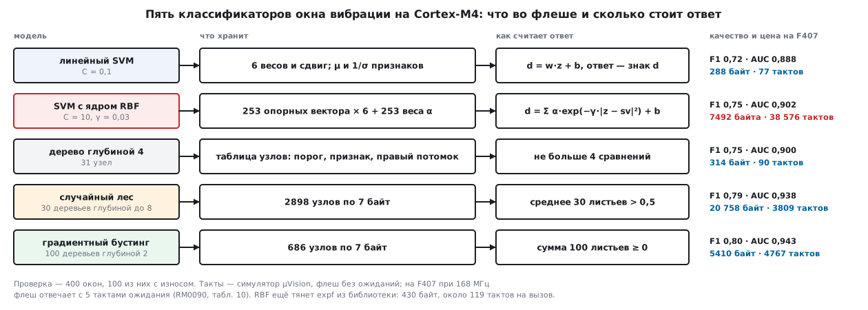
The second task is to decide from a vibration window whether the bearing is healthy or worn. Six window features, as in section 117: RMS, peak frequency, crest factor, energy share in the band, kurtosis and the housing temperature. Wear raises the crest factor, the kurtosis and the band energy slightly. But in a healthy motor the band energy also rises in a hump as the speed passes the housing resonance — the boundary between the classes is curved:
band = 0.06 + 0.25 * np.exp(-((v - 0.55) / 0.12) ** 2) + 0.14 * s + rc.normal(0, 0.02, n)
Sets: 600 windows for training (200 worn), 400 for testing (100 worn) and another 4000 "new motors" for experiments, on which nothing is chosen.
Wear is a rare and costly class, and the share of correct answers says nothing about it. The answers are split into four numbers: wear found correctly (TP), a false alarm (FP), wear missed (FN), "healthy" said correctly (TN). From them:
- recall = TP / (TP + FN) — the share of worn bearings found;
- precision = TP / (TP + FP) — the share of alarms that are real;
- F1 = 2·TP / (2·TP + FP + FN) — one number that drops if either of the two is poor.
| Model | TP | FP | FN | Recall | Precision | F1 | AUC |
|---|---|---|---|---|---|---|---|
| Linear SVM | 65 | 15 | 35 | 65 % | 81.3 % | 0.72 | 0.888 |
| RBF SVM | 65 | 9 | 35 | 65 % | 87.8 % | 0.75 | 0.902 |
| Depth-4 tree | 72 | 20 | 28 | 72 % | 78.3 % | 0.75 | 0.900 |
| Random forest | 76 | 17 | 24 | 76 % | 81.7 % | 0.79 | 0.938 |
| Gradient boosting | 80 | 20 | 20 | 80 % | 80.0 % | 0.80 | 0.943 |
Every model outputs not only a class but also a number — the distance to the boundary for an SVM, the vote share for a forest, the sum for boosting — and the class comes from comparing it with a threshold. Moving the threshold trades recall for precision. The ROC curve is the share of wear found against the share of false alarms over all thresholds at once, and AUC is the area under it: 1 means the model always ranks a worn bearing above a healthy one, 0.5 means it guesses. AUC does not depend on the chosen threshold and is handy for comparing models. For boosting, a threshold of −1 instead of 0 finds 89 worn bearings out of 100 instead of 80, but gives 55 false alarms instead of 20, and precision drops to 61.8 %. Where to put the threshold is decided by the cost of the errors, as in section 116.7.
116а.4 The support vector machine
A linear SVM looks for a plane w·z + b = 0 with the largest gap between it and the nearest examples of both classes. The examples on the edge of the gap and inside it are the support vectors: they alone define the plane. The classes overlap, so the margin is soft: an example may cross the edge at a price proportional to C. A small C gives a wide margin and many support vectors, a large one gives a narrow margin fitted tightly to the training data:
| C | 0.01 | 0.1 | 1 | 10 |
|---|---|---|---|---|
| Support vectors out of 600 | 330 | 276 | 266 | 266 |
| Correct out of 400 | 348 | 350 | 349 | 349 |
Cross-validation chose C = 0.1. For the linear kernel the board does not need the support vectors: they fold into 6 weights, and inference is a dot product:
    for (int i = 0; i < N_FEAT; i++)
        d += LIN_W[i] * z[i];
    return d > 0.0f;
288 bytes and 77 cycles, 350 correct out of 400. But a plane cannot follow the hump of the band energy, and recall is 65 %.
The RBF kernel replaces the dot product with the similarity exp(−γ·|z − sv|²): the boundary becomes curved, but the support vectors no longer fold. The answer is a sum over all of them:
    for (int k = 0; k < N_SV; k++) {
        const float *sv = &SV[k * N_FEAT];
        float r2 = 0.0f;
        for (int i = 0; i < N_FEAT; i++) {
            float t = z[i] - sv[i];
            r2 += t * t;
        }
        d += SV_ALPHA[k] * expf(-RBF_GAMMA * r2);
    }
Cross-validation chose C = 10 and γ = 0.03; there are 253 support vectors out of 600. The model drags almost half of the training set into flash: 6072 bytes of vectors, 1012 bytes of α weights and expf from the library — another 430 bytes. An answer costs 38 576 cycles, about 150 cycles per support vector, while a single expf in a separate loop takes about 119 cycles. At 168 MHz that is about 230 µs without flash wait states — 500 times the linear SVM for 6 more correct answers out of 400 and F1 0.75 instead of 0.72. The number of support vectors grows with the training set, like the memory of k nearest neighbours in section 116.5.
116а.5 Ensembles: forest and boosting
A single deep tree memorises the training set: a tree without a limit grew to depth 16 and 157 nodes, 600 out of 600 correct on training and only 344 out of 400 on the test set. The depth-4 tree chosen by cross-validation gets 352 out of 400. A deep tree is not bad but unstable: another training set gives other thresholds and other errors.
Bagging exploits this. Each tree learns on its own random sample, drawn with replacement from the training set, and in a random forest each node also picks its threshold from a random subset of the features. The trees' errors become different, and averaging cancels part of them. scikit-learn averages not the votes but the class shares in the leaves — "soft" voting. A forest of full trees on 4000 new windows:
| Trees | 1 | 3 | 10 | 30 | 100 |
|---|---|---|---|---|---|
| Correct out of 4000 | 3139 | 3299 | 3435 | 3482 | 3487 |
| Nodes in total | 141 | 423 | 1486 | 4250 | 14088 |
One tree of the forest is worse than a single full tree (3212 out of 4000): it did not see all the examples. From 30 trees on, the gain almost stops while the memory keeps growing: 100 full trees are 14088 nodes, at 7 bytes per node that is 98 616 bytes of flash for 5 more correct answers out of 4000. The firmware takes a forest of 30 trees of depth up to 8 (cross-validation chose the depth): 2898 nodes, 359 correct out of 400 and 3510 out of 4000.
Boosting builds the trees not independently but one after another: each next tree — small, of depth 2 — learns to correct the errors of the sum of the previous ones, and its contribution is multiplied by a step of 0.1. The answer is the sign of the sum:
    float s = GB_INIT;
    for (int t = 0; t < N_TREES_GB; t++)
        s += walk(GB_THR, GB_FEAT, GB_RIGHT, GB_ROOT[t], x);
    return s >= 0.0f;
100 trees of 2 comparisons each — 686 nodes, 360 correct out of 400 and 3536 out of 4000: better than the forest with an almost four times smaller table. The forest cancels the scatter of deep trees, boosting adds up many weak ones — and both follow the hump of the band energy in steps, which a plane cannot do.
116а.6 Export to C and the comparison table
The weights of the linear models and the support vectors go into the header as
float arrays. Trees go as a node table: the threshold, the feature number and
the number of the right child; the left child is always the next node, because
scikit-learn numbers the nodes in depth-first order. A leaf has the feature
number −1, and its threshold field holds its value — the share of wear for the
tree and the forest, the contribution for boosting. A node is 7 bytes:
    while (feat[n] >= 0)
        n = x[feat[n]] <= thr[n] ? n + 1 : right[n];
    return thr[n];                      /* у листа в thr лежит его значение */
At export the threshold is rounded to the largest float not greater than the
scikit-learn threshold: then x <= thr[n] gives the same branch for any float
x. With rounding to nearest, 504 thresholds out of 1742 would become larger than
the real ones; on the 400 and 4000 windows this did not change a single answer,
but a window lying exactly on such a value would go down the other branch.
The check: the same infer116b.c, built with gcc on the computer and with
armclang for the F407 in the µVision simulator, answered like scikit-learn in all
400 windows for all five classifiers. Flash is the function and its tables from
the armclang -O2 object file; cycles are the simulator counter over all 400
windows, minus an empty pass of the loop:
| Model | Correct out of 400 | F1 | AUC | Flash, bytes | Cycles per answer |
|---|---|---|---|---|---|
| Linear SVM | 350 | 0.72 | 0.888 | 288 | 77 |
| RBF SVM | 356 | 0.75 | 0.902 | 7492 + expf 430 | 38 576 |
| Depth-4 tree | 352 | 0.75 | 0.900 | 314 | 90 |
| Random forest, 30 trees | 359 | 0.79 | 0.938 | 20 758 | 3809 |
| Boosting, 100 trees of depth 2 | 360 | 0.80 | 0.943 | 5410 | 4767 |
The winding temperature regression: RMSE 1.00 °C, 212 bytes, 39 cycles. The simulator models flash without wait states. On the F407 at 168 MHz the flash answers with 5 wait states (RM0090, table 10). The ART accelerator — an instruction prefetch queue and a branch cache — gives, by CoreMark, the speed of zero wait states (RM0090, 3.5.2), but the node tables and support vectors are read as data and out of order; how much the cycle counts grow on the board was not measured.
116а.7 Pitfalls
An SVM on raw features does worse than the linear one. The RBF kernel measures distance, and a temperature in tens of degrees drowns an energy share in tenths. Without standardization the same SVM is right in 329 cases out of 400 instead of 356 and finds 55 worn bearings out of 100 instead of 65. The mean and spread are computed on the training set — separately inside each cross-validation fold — and shipped into the firmware.
The tree is right on every training example. Unlimited depth: 600 out of 600 on training and 344 out of 400 on the test set. Limit the depth by cross-validation or use a forest.
Hyperparameters tuned on the test set. The experiment was repeated on 50 test sets of 400 windows: an SVM with the C and γ best on the test set shows on it 88.34 % on average, while on 10 000 windows nobody has seen — 87.57 %. The one chosen by cross-validation shows 86.74 % on the test set and 86.95 % on new data: its estimate is honest. The inflation is small — 0.77 points against a spread of 1.96 points from one set to another — but always in the same direction. Tune by cross-validation on the training set, test once at the end.
The forest does not fit into flash. Nodes grow with the number and depth of the trees: 100 full trees take 98 616 bytes. Limit the depth and take the number of trees where the quality curve reaches its plateau.
RBF cannot keep up with the window. 38 576 cycles per answer and a number of support vectors that grows with the data. First try a feature that straightens the boundary — like q in 116а.1 — and a linear model.
Gradient descent does not converge. Features of different scale: a step that is stable for a speed in thousands does nothing to the rest.
116а.8 Summary
- Linear regression: least squares in closed form, RMSE 2.48 °C on raw features and 1.00 °C with the feature q — down to the sensor noise; in C — 212 bytes and 39 cycles.
- Gradient descent: 865 steps on standardized features; without scaling the condition number is 87281598 and RMSE is 7.86 °C after 10 000 steps.
- Ridge on 12 examples with two current sensors: λ = 0.1 gives weights −1.09 and 0.08 instead of −10.84 and 6.62, RMSE 1.16 °C instead of 2.47.
- Metrics for a rare class are recall, precision and F1; AUC compares models without choosing a threshold.
- Linear SVM — 288 bytes and 77 cycles, F1 0.72; RBF — 253 support vectors, 7492 bytes and 38 576 cycles, F1 0.75.
- A forest of 30 trees — F1 0.79, 20 758 bytes; boosting with 100 trees of depth 2 — F1 0.80, 5410 bytes and 4767 cycles.
- The C answers matched scikit-learn in all 400 windows for all five models.
- Standardize features for an SVM, limit tree depth, tune hyperparameters only by cross-validation.
Full sources
infer116b.c — inference of the regression and five classifiers in C, in float, with parameters from model116b.h.
/* Раздел 116а: регрессия, SVM, дерево, лес и бустинг — вывод на Cortex-M4F во float.
* Параметры — из model116b.h (выгрузил train116b.py). Регрессия берёт воздух, °C,
* ток, А, и обороты, об/мин, и отвечает температурой обмотки, °C. Классификаторы
* берут шесть признаков окна вибрации и отвечают: 0 — исправен, 1 — износ.
* На компьютере main сверяет ответы с scikit-learn (-DML_HOST).
* Проверка — _verify/ml116b_check.py. */
#include <math.h>
#include "model116b.h"
/* 1. Линейная регрессия: признак q = I²/(1 + n/1000), затем скалярное произведение */
float reg_predict(const float x[3])
{
const float f[4] = { x[0], x[1], x[2], x[1] * x[1] / (1.0f + x[2] / 1000.0f) };
float y = REG_B;
for (int i = 0; i < 4; i++)
y += REG_W[i] * (f[i] - REG_MU[i]) * REG_INV_SD[i];
return y;
}
static void standardize(const float x[N_FEAT], float z[N_FEAT])
{
for (int i = 0; i < N_FEAT; i++)
z[i] = (x[i] - MU[i]) * INV_SD[i];
}
/* 2. Линейный SVM: знак скалярного произведения */
int svm_lin_predict(const float x[N_FEAT])
{
float z[N_FEAT], d = LIN_B;
standardize(x, z);
for (int i = 0; i < N_FEAT; i++)
d += LIN_W[i] * z[i];
return d > 0.0f;
}
/* 3. SVM с ядром RBF: сумма по всем опорным векторам */
int svm_rbf_predict(const float x[N_FEAT])
{
float z[N_FEAT], d = RBF_B;
standardize(x, z);
for (int k = 0; k < N_SV; k++) {
const float *sv = &SV[k * N_FEAT];
float r2 = 0.0f;
for (int i = 0; i < N_FEAT; i++) {
float t = z[i] - sv[i];
r2 += t * t;
}
d += SV_ALPHA[k] * expf(-RBF_GAMMA * r2);
}
return d > 0.0f;
}
/* Спуск по таблице узлов: левый потомок — следующий узел, правый — по номеру */
static float walk(const float *thr, const signed char *feat, const unsigned short *right,
unsigned n, const float x[N_FEAT])
{
while (feat[n] >= 0)
n = x[feat[n]] <= thr[n] ? n + 1 : right[n];
return thr[n]; /* у листа в thr лежит его значение */
}
/* 4. Дерево: в листе — доля износа среди обучающих примеров */
int tree_predict(const float x[N_FEAT])
{
return walk(TREE_THR, TREE_FEAT, TREE_RIGHT, 0, x) > 0.5f;
}
/* 5. Случайный лес: средняя доля по деревьям */
int forest_predict(const float x[N_FEAT])
{
float s = 0.0f;
for (int t = 0; t < N_TREES_RF; t++)
s += walk(RF_THR, RF_FEAT, RF_RIGHT, RF_ROOT[t], x);
return s > 0.5f * N_TREES_RF;
}
/* 6. Градиентный бустинг: сумма маленьких деревьев, знак — ответ */
int boost_predict(const float x[N_FEAT])
{
float s = GB_INIT;
for (int t = 0; t < N_TREES_GB; t++)
s += walk(GB_THR, GB_FEAT, GB_RIGHT, GB_ROOT[t], x);
return s >= 0.0f;
}
#ifdef ML_HOST
#include <stdio.h>
int main(void)
{
static const struct {
const char *name;
int (*fn)(const float *);
const unsigned char *sk;
} m[5] = {
{ "lin", svm_lin_predict, SK_LIN }, { "rbf", svm_rbf_predict, SK_RBF }, { "tree", tree_predict, SK_TREE },
{ "rf", forest_predict, SK_RF }, { "gb", boost_predict, SK_GB },
};
double worst = 0.0;
for (int i = 0; i < N_REG_TEST; i++) {
double e = fabs((double)reg_predict(®_TEST_X[3 * i]) - REG_SK[i]);
worst = e > worst ? e : worst;
}
printf("c_reg=%.6f\n", worst);
for (int k = 0; k < 5; k++) {
int same = 0, right = 0;
for (int i = 0; i < N_TEST; i++) {
int p = m[k].fn(&TEST_X[N_FEAT * i]);
same += p == m[k].sk[i];
right += p == TEST_Y[i];
}
printf("c_%s=%d,%d\n", m[k].name, same, right);
}
printf("done=1\n");
return 0;
}
#endif
Next: section 116б "How a neural network learns: the neuron, activation functions, the loss function, backpropagation, gradient descent, SGD, momentum and Adam" — what is inside the line "train the network": the chain rule by hand, the learning rate, Adam and overfitting, from scratch in numpy.