 Embedded HandbookApps
116б. How a neural network learns: the neuron, activation functions, the loss function, backpropagation, gradient descent, SGD, momentum and Adam
In 116.6 the perceptron was trained by scikit-learn in one line, in 118 the same way, in 119 by TensorFlow. Here that line is taken apart: what a neuron computes, how the error is measured, how the chain rule gives the gradient of every weight, why descent with momentum and Adam beat a plain step, and why a network overfits. Everything is written from scratch in numpy, without a framework, on a task with two pump sensors. The trained 2 → 16 → 3 network then goes to C: bytes on the F407, instructions per answer in QEMU, and C answers checked against numpy.
Sources: numpy 2.3.3 in the stm-ml:1 image, the train116c.py script —
every number in the section comes from its run, and a rerun produces the same files.
The C inference is built with gcc 12.2.0 (stm-sys:1) for the cross-check, with armclang 6.24 for
the F407 for sizes, and with arm-none-eabi-gcc 12.2.1 and QEMU 7.2 (stm-arm:1, the
netduinoplus2 board with an STM32F405) to count instructions.
Terms used in the documentation
Term Meaning neuron, weight, bias a weighted sum of inputs plus an offset activation function the non-linear function applied to that sum sigmoid, tanh, ReLU the logistic curve, the hyperbolic tangent, the "rectifier" max(0, x) forward pass from the input to the answer logits the network outputs before softmax loss function one number for "how bad" mean squared error (MSE) the average of the squared error cross-entropy minus the log of the probability of the right class backpropagation carrying the error back from the output to the input gradient check comparing the gradient with finite differences learning rate the size of the descent step epoch, mini-batch an epoch is one pass over the whole set; a batch is the part of it used for one step stochastic gradient descent (SGD) a step on each batch momentum the step accumulates speed Adam descent with momentum and its own step scale for every weight Xavier (Glorot), He initialization initial weights with a spread set by the number of inputs vanishing gradient the gradient fades towards the first layers overfitting, regularization learning the examples instead of the rule, and the remedies weight decay (L2), dropout, early stopping a penalty on large weights, switching neurons off, stopping at the best epoch
116б.1 The neuron, the layer, the forward pass
The task: a centrifugal pump, a pressure sensor on the outlet (bar) and a flow meter (l/min). A healthy pump sits on the rated curve P = 4,0 · (1 − (Q/60)²); a worn impeller gives less head at the same flow. Three classes: normal — 92…104 % of the rated head, wear — 74…88 %, severe wear or air ingress — 50…66 %. The pressure sensor noise is 0,05 bar, the flow meter noise 0,6 l/min. The data are synthetic, with a fixed seed: 600 examples for training, 300 for tuning and 300 for testing, one third per class. The boundary between the classes is a curve; a straight line cannot draw it.
A neuron is a weighted sum of the inputs plus a bias, passed through an activation function: h = f(w₁x₁ + w₂x₂ + b). A layer of 16 neurons is a 2 × 16 weight matrix: a = W·z + b, one multiplication for all neurons at once. The forward pass goes layer by layer from the input to the logits:
    for (int j = 0; j < N_HID; j++) {
        float a = NN_B1[j];
        for (int i = 0; i < N_IN; i++)
            a += z[i] * NN_W1[i * N_HID + j];          /* a = W·z + b */
        h[j] = a > 0.0f ? a : 0.0f;                    /* ReLU */
    }
The 2 → 16 → 3 network has 99 parameters and 80 multiplications per answer. Without an activation function two layers collapse into one: a product of matrices is again a matrix, and the network stays a straight boundary.
Activation functions. The step (0 or 1) is the most direct "fired or not", but its derivative is zero everywhere — there is no gradient and nothing to learn with. The sigmoid 1/(1 + e⁻ˣ) is smooth, but its derivative is at most 0,25, and at x = 4 only 0,0177. For tanh the largest derivative is 1, at x = 4 it is 0,0013. ReLU = max(0, x): the derivative is 1 for any x > 0, and it costs one comparison on the device. The same 2 → 16 → 3 network, Adam, 60 epochs, different activations in the hidden layer:
| Hidden layer | Training loss | Correct out of 300 |
|---|---|---|
| none (output directly, straight boundaries) | 0,4123 | 260 |
| sigmoid | 0,1900 | 276 |
| tanh | 0,0837 | 287 |
| ReLU | 0,0605 | 290 |
116б.2 The loss function: MSE for a number, cross-entropy for classes
To descend, you need one number for "how bad" and its derivative with respect to every output.
A number — the mean squared error. L = mean (ŷ − y)², the derivative with respect to the output is 2(ŷ − y)/N. Example: estimate what percentage of the rated head the pump delivers. The linear 2 → 1 model is off on the test set on average (root mean square) by 6,85 %, at the worst point by 22,38 %; the 2 → 16 → 1 network by 3,04 % and 12,13 %: a straight line cannot follow the curve of the rated characteristic.
A class — softmax and cross-entropy. The three logits are turned into probabilities pᵢ = e^sᵢ / Σ e^sⱼ, the loss is minus the log of the probability of the right class. Logits (2; 1; 0,1) give probabilities 0,659; 0,242; 0,099: if the first class is right, the loss is 0,417, if the third, 2,317. A network that answers "all three are equal" has a loss of ln 3 = 1,0986; our network with random initial weights has 1,4452. The derivative with respect to the logits for the softmax + cross-entropy pair is simple — p − y:
def ce_loss(s, y):
    """Перекрёстная энтропия после softmax и её градиент по логитам: (p − y) / N."""
    lp = log_softmax(s)
    n = len(y)
    g = np.exp(lp)
    g[np.arange(n), y] -= 1.0
    return -lp[np.arange(n), y].mean(), g / n
116б.3 Backpropagation: the chain rule by hand
For a two-layer network a₁ = W₁z + b₁, h = f(a₁), s = W₂h + b₂ the derivatives go from the output to the input; every link is one derivative:
- with respect to the logits: δ₂ = (p − y)/N;
- with respect to the output layer weights: ∂L/∂W₂ = hᵀ·δ₂, to the bias — the sum of δ₂;
- into the hidden layer: ∂L/∂h = δ₂·W₂ᵀ;
- through the activation: δ₁ = ∂L/∂h ⊙ f′(a₁) — for ReLU this just zeroes it where a₁ ≤ 0;
- with respect to the first layer weights: ∂L/∂W₁ = zᵀ·δ₁.
    for i in range(len(P) - 1, -1, -1):
        h_in, a, hn, mask = cache[i]
        if i < len(P) - 1:                        # через активацию: dL/da = dL/dh · f'(a)
            if mask is not None:
                g = g * mask
            if not bug:
                g = g * df(a, hn if mask is None else ACT[act][0](a))
        W = P[i][0]
        grads[i] = [h_in.T @ g + 2.0 * l2 * W, g.sum(axis=0)]
        g = g @ W.T                               # в предыдущий слой
Your own backward pass must be checked. Finite differences: shift one weight by ±10⁻⁵, compute the loss twice, divide the difference by 2·10⁻⁵ — and do this for every weight. On 5 examples, for the 2 → 4 → 3 network (27 parameters) the largest relative difference from the formulas is 2,4·10⁻¹⁰, for the 2 → 4 → 1 network with MSE (17 parameters) 7,1·10⁻¹¹. A deliberately forgotten ReLU derivative gives 1,0: the check catches the error at once. The device has no backward pass — it is needed only for training.
116б.4 Gradient descent: the step, SGD, momentum and Adam
A descent step: w ← w − η·∂L/∂w. The key here is the learning rate η. Descent on the whole set (one step per epoch), 300 epochs, the same starting point:
| Rate η | Loss after 300 epochs | Correct out of 300 | Largest loss on the way |
|---|---|---|---|
| 0,01 | 0,6497 | 230 | 1,5437 |
| 0,1 | 0,2108 | 288 | 1,3793 |
| 1 | 0,0707 | 289 | 1,1649 |
| 3 | 0,0744 | 282 | 2,7296 |
| 10 | 1,3947 | 100 | 2,2 million |
Too small is slow: at 0,01 the network did not even reach 0,6 in 300 epochs. Too large jumps: at 3 the loss rose to 2,73 on the way, at 10 to millions, and the network collapsed into one class (100 out of 300 — exactly one third).
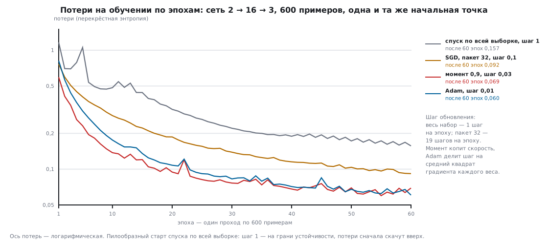
SGD. The gradient over a batch of 32 examples is a noisy but cheap estimate of the full one: 19 steps per epoch instead of 1. Momentum accumulates speed: v ← 0,9·v + g, w ← w − η·v — in a steady direction the step grows, across oscillations it is damped. Adam keeps two averages — of the gradient and of its square — and divides one by the root of the other: every weight gets its own step scale.
                    elif opt == "momentum":
                        st[li][q] = 0.9 * st[li][q] + G[li][q]
                        step = lr * st[li][q]
                    else:                                       # Adam: β1 0,9, β2 0,999
                        st[li][q] = 0.9 * st[li][q] + 0.1 * G[li][q]
                        st2[li][q] = 0.999 * st2[li][q] + 0.001 * G[li][q] ** 2
                        mh = st[li][q] / (1 - 0.9 ** t)
                        vh = st2[li][q] / (1 - 0.999 ** t)
                        step = lr * mh / (np.sqrt(vh) + 1e-8)
| Method | Rate | Loss after 10 epochs | After 60 epochs | Epochs to loss < 0,2 | Correct out of 300 |
|---|---|---|---|---|---|
| descent on the whole set | 1 | 0,4840 | 0,1569 | 35 | 286 |
| SGD, batch 32 | 0,1 | 0,2819 | 0,0917 | 18 | 289 |
| momentum 0,9, batch 32 | 0,03 | 0,1375 | 0,0694 | 6 | 288 |
| Adam, batch 32 | 0,01 | 0,1757 | 0,0605 | 9 | 290 |
Adam gave the lowest loss after 60 epochs and the best test result; the same Adam with rate 0,01 trains the network in 119, and in section 118а the same mechanics is hidden inside Keras.
116б.5 Initialization, the vanishing gradient, overfitting
Not with zeros. All weights zero — ReLU has neither output nor gradient: the loss stays at 1,0986 = ln 3, the network answers with one class (100 out of 300). All weights equal (0,5) — the 16 neurons get the same gradient and remain copies of one: after training there is 1 distinct neuron, and 256 out of 300 are correct. Randomness breaks this symmetry, and the spread is chosen by the number of inputs: Xavier — σ = √(2/(n_in + n_out)) for the sigmoid and tanh, He — σ = √(2/n_in) for ReLU.
A deep network. Ten hidden layers of 32 neurons, the initial weights, one gradient estimate on 600 examples:
| Network | Signal spread: 1st layer / 10th | Weight gradient: 1st layer / output |
|---|---|---|
| sigmoid, Xavier | 7,55·10⁻² / 1,28·10⁻¹ | 8,43·10⁻⁸ / 7,30·10⁻¹ |
| tanh, Xavier | 2,74·10⁻¹ / 1,54·10⁻¹ | 1,07·10⁻¹ / 2,61·10⁻¹ |
| ReLU, He | 7,92·10⁻¹ / 1,34 | 5,04·10⁻¹ / 3,48 |
| ReLU, σ = 1 | 7,92·10⁻¹ / 3,51·10⁵ | 5,21·10⁵ / 1,61·10⁶ |
| ReLU, σ = 0,01 | 7,92·10⁻³ / 3,51·10⁻¹⁵ | 2,62·10⁻¹⁵ / 2,67·10⁻¹⁵ |
With the sigmoid the first-layer gradient is millions of times smaller than the output one: at every layer it is multiplied by the derivative of the sigmoid, which is at most 0,25. This is the vanishing gradient. SGD, rate 0,1, 30 epochs: the sigmoid network moved the loss from 1,1215 only to 1,1017 and answers with one class (100 out of 300); the same network with ReLU and He went from 0,8048 to 0,1448, 279 correct. Weights that are too large blow the signal up, weights that are too small damp it to zero.
Overfitting. Little data and a big network: 60 examples (20 per class), a 2 → 64 → 64 → 3 network (4547 parameters), Adam, 1500 epochs. The network learns all 60 examples, the loss on them is zero, but on the test set it is worse than the small network on 600 examples (292, 116б.6):
| Method | Correct in training out of 60 | Correct in test out of 300 | Training loss | Test loss |
|---|---|---|---|---|
| no regularization | 60 | 278 | 0,0000 | 0,3618 |
| L2, λ = 0,003 | 60 | 283 | 0,0459 | 0,1449 |
| dropout 0,3 | 60 | 276 | 0,0005 | 0,3606 |
| early stopping (epoch 95) | 60 | 276 | 0,0367 | 0,1567 |
L2 penalizes large weights and gives the best result. Early stopping takes the weights from the epoch where the loss on the tuning set (300 examples, not used in training) was lowest: the test loss fell from 0,3618 to 0,1567. Dropout did not help here (276 against 278): a regularization technique is checked on the tuning set like any other. The best remedy is more data.
116б.6 On the Cortex-M4: C inference, bytes and instructions
The final 2 → 16 → 3 network: Adam, rate 0,01, batch 32, up to 200 epochs, early stopping chose epoch 171. Correct: 594 out of 600 in training, 294 out of 300 in tuning and 292 out of 300 in testing. Severe wear is recognized in all 100 cases; the network took normal for wear 6 times, and wear once for normal and once for severe wear.
On the device softmax is not needed for the decision: the index of the largest logit is the same. Probabilities are computed only when confidence is needed, and then the largest logit is subtracted first:
    for (int c = 0; c < N_OUT; c++) {
        p[c] = expf(s[c] - m);
        sum += p[c];
    }
The cross-check. The weights, the input mean and spread are exported to model116c.h
as float. The same infer116c.c, built with gcc on the computer, gave on
the 300 test examples the same classes as numpy in 300 cases out of 300;
the logits differed by at most 1,1·10⁻⁵ (C computes in float,
numpy in double), the probabilities by 1,9·10⁻⁶. In QEMU on the Cortex-M4F —
also 300 out of 300.
Bytes on the F407 (armclang, -mcpu=cortex-m4 -mfpu=fpv4-sp-d16):
-O2 |
-Os |
|
|---|---|---|
nn_forward |
1196 bytes | 228 bytes |
nn_classify |
56 bytes | 54 bytes |
nn_probs |
132 bytes | 116 bytes |
| object code with literals | 1588 bytes | 498 bytes |
| constant tables | 216 bytes | 344 bytes |
There are 103 weights and normalization numbers, which is 412 bytes of flash. With -O2
the compiler unrolled the loops — nn_forward has 64 VMUL.F32 instructions
in a row, and some weights went into the literal pool inside the code; with -Os the loops
stayed loops. RAM is only the arrays on the stack: z, h and s, 21 numbers.
Instructions per answer — QEMU netduinoplus2 with -icount, SysTick counts,
code by arm-none-eabi-gcc -O2: nn_classify — 677 instructions per call including
the test loop, nn_probs with expf — 903. These are instructions, not cycles: there are more cycles
on the chip, so the time below is a lower bound. At 168 MHz it is
at least 4,0 µs per answer.
What other networks there are — briefly, details in their own sections:
| Architecture | What it does | On a microcontroller | Where in the handbook |
|---|---|---|---|
| dense (fully connected) | every input is connected to every neuron | features from sensors: from a few to tens of inputs | 116.6, 118, this section; Keras — section 118а; int8 — 119 |
| convolutional | one small filter slides over the signal or the image | sound spectrograms, images | 121б (sound), 121в (camera with an NPU) |
| recurrent | keeps a state between the steps of a series | long series; in this part a window with features replaces it (117) | — |
| autoencoder | compresses and restores the input; the restoration error measures "not like that" | anomaly detection, learns only from normal data | 120 (64 → 8 → 64) |
| transformer | every step of a series looks at all the others | large models; not used in this part | — |
116б.7 Pitfalls
The network does not learn: the loss is stuck around 1. The input is not normalized: the flow is in tens of l/min, the pressure in units of bar. Without normalization SGD over 60 epochs: rate 0,1 — loss 1,0295 and 125 correct out of 300, rate 0,01 — 0,9996 and 146, rate 0,001 — 2,0561 and 100. With normalization the same SGD reaches 0,0917 and 289. The mean and spread are part of the model; they go into the firmware together with the weights.
NaN in the probabilities. expf in float already overflows at 89
(e⁸⁸ is still finite). Logits (1000; 999; 0) computed head-on give two NaN out of three,
after subtracting the largest one — 0,7311; 0,2689; 0,0000. The same in numpy:
log_softmax starts with s - s.max(...).
The loss jumps up, then NaN. The learning rate is too large: at 10 — millions (116б.4). Reduce the rate until the curve is smooth, or take Adam with 0,01.
SGD learns worse than descent on the whole set. The data are not shuffled: the examples lie by class, and consecutive batches pull the network towards one class, then towards another. Without shuffling, after 60 epochs the loss is 0,1475 and 272 correct; with shuffling every epoch — 0,0917 and 289.
Your own backward pass "almost works". An error in a gradient formula is invisible by eye: the loss is computed by the forward pass, and that one is correct. The finite-difference check shows 1,0 instead of 10⁻¹⁰ — run it on every new formula.
All the neurons are the same. The weights were started at zero or at one constant — only random initialization breaks the symmetry (116б.5).
116б.8 Summary
- A neuron is a weighted sum plus a bias and an activation; a layer is a multiplication by a matrix. The 2 → 16 → 3 network has 99 parameters and 80 multiplications.
- ReLU: the derivative is 1 over the whole positive half; for the sigmoid it is at most 0,25. On the pump task ReLU gives 290 correct out of 300, the sigmoid 276, no hidden layer 260.
- Losses: MSE for a number (the network 3,04 % against 6,85 % for the straight line), cross-entropy with softmax for classes, the gradient with respect to the logits is p − y.
- Backpropagation is the chain rule from the output to the input; finite differences agree with the formulas to 2,4·10⁻¹⁰, a forgotten derivative gives 1,0.
- Rate 0,01 is slow, 10 diverges. After 60 epochs: descent on the whole set — 0,1569, SGD — 0,0917, momentum — 0,0694, Adam — 0,0605.
- Zero weights — the network does not learn; the sigmoid in 10 layers damps the gradient of the first layer to 8,43·10⁻⁸.
- 60 examples for a network with 4547 parameters is overfitting; L2 raised the test result from 278 to 283, the best is 600 examples and a small network: 292.
- On the F407: 412 bytes of weights,
nn_forwardis 228 bytes with-Os; 677 instructions per answer, at least 4,0 µs at 168 MHz; the C answers matched numpy in 300 cases out of 300.
Full sources
infer116c.c — C inference of the network in float with weights from model116c.h.
/* Раздел 116б: обученная на numpy сеть 2 → 16 → 3 — вывод на Cortex-M4F во float.
 * Веса — из model116c.h (выгрузил train116c.py). Вход — расход, л/мин, и давление, бар,
 * ответ — класс: 0 — норма, 1 — износ колеса, 2 — сильный износ или подсос воздуха.
 * На компьютере (-DML_HOST) main сверяет классы, логиты и вероятности с numpy
 * на проверочной выборке. Проверка — _verify/ml116c_check.py. */
#include <math.h>
#include <stdint.h>

#if defined(ML_HOST) && !defined(ML_DATA)
#define ML_DATA
#endif
#include "model116c.h"

/* Прямой проход: нормировка, скрытый слой с ReLU, выходной слой — логиты */
void nn_forward(const float x[N_IN], float s[N_OUT])
{
    float z[N_IN], h[N_HID];
    for (int i = 0; i < N_IN; i++)
        z[i] = (x[i] - NN_MU[i]) / NN_SD[i];           /* среднее и разброс — часть модели */
    for (int j = 0; j < N_HID; j++) {
        float a = NN_B1[j];
        for (int i = 0; i < N_IN; i++)
            a += z[i] * NN_W1[i * N_HID + j];          /* a = W·z + b */
        h[j] = a > 0.0f ? a : 0.0f;                    /* ReLU */
    }
    for (int c = 0; c < N_OUT; c++) {
        float a = NN_B2[c];
        for (int j = 0; j < N_HID; j++)
            a += h[j] * NN_W2[j * N_OUT + c];
        s[c] = a;
    }
}

/* Класс — номер наибольшего логита: softmax его не меняет и на приборе не нужен */
int nn_classify(const float x[N_IN])
{
    float s[N_OUT];
    nn_forward(x, s);
    int k = 0;
    for (int c = 1; c < N_OUT; c++)
        if (s[c] > s[k])
            k = c;
    return k;
}

/* Вероятности — когда нужна уверенность: сначала вычесть наибольший логит, иначе expf переполнится */
void nn_probs(const float x[N_IN], float p[N_OUT])
{
    float s[N_OUT], m, sum = 0.0f;
    nn_forward(x, s);
    m = s[0];
    for (int c = 1; c < N_OUT; c++)
        m = s[c] > m ? s[c] : m;
    for (int c = 0; c < N_OUT; c++) {
        p[c] = expf(s[c] - m);
        sum += p[c];
    }
    for (int c = 0; c < N_OUT; c++)
        p[c] /= sum;
}

#ifdef ML_HOST
#include <stdio.h>

int main(void)
{
    int same = 0, right = 0;
    float dl = 0.0f, dp = 0.0f;
    for (int i = 0; i < N_TEST; i++) {
        float s[N_OUT], p[N_OUT];
        int k = nn_classify(&TEST_X[N_IN * i]);
        nn_forward(&TEST_X[N_IN * i], s);
        nn_probs(&TEST_X[N_IN * i], p);
        same += k == NP_CLASS[i];
        right += k == TEST_Y[i];
        for (int c = 0; c < N_OUT; c++) {
            float e = fabsf(s[c] - NP_LOGIT[N_OUT * i + c]), f = fabsf(p[c] - NP_PROB[N_OUT * i + c]);
            dl = e > dl ? e : dl;
            dp = f > dp ? f : dp;
        }
    }
    printf("agree=%d,%d\nright=%d\n", same, N_TEST, right);
    printf("max_dlogit=%.1e\nmax_dprob=%.1e\n", (double)dl, (double)dp);
    return 0;
}
#endif
Next: section 117 "Data from the sensor: windows, features, CMSIS-DSP" — where the RMS and the peak frequency come from.