 Embedded HandbookApps
116. Typical approaches and algorithms: from a threshold to a small neural network
On a microcontroller, "machine learning" almost always means one thing: from
a few numbers from a sensor, decide what state the object is in. There are
five typical approaches for this — a threshold, logistic regression, a decision
tree, k nearest neighbours and a small neural network. This section solves one
task with all of them — the state of a motor from its vibration — and compares them by accuracy,
memory, number of multiplications and code size on the F407. Training is scikit-learn
in the stm-ml:1 image, inference is our own C code, and its answers match
scikit-learn on the whole test set.
TinyML in general is section 85, features from the signal are section 117, training is section 118.
Terms used in the documentation
Term Meaning feature a number the decision is based on class, label the category an example belongs to, its tag training set, test set the examples the model learns from and the ones it is checked on accuracy the share of correct answers inference getting an answer from a trained model threshold rule a fixed cut-off, a hand-written rule logistic regression a weighted sum per class, the largest one wins decision tree a chain of comparisons, one per level k-nearest neighbours (k-NN) a vote of the k closest stored examples multilayer perceptron (MLP) a small neural network with hidden layers ReLU a "rectifier": max(0, x) standardization scaling a feature to mean 0 and spread 1 multiply-accumulate (MAC) a multiplication followed by an addition
116.1 The task and the data
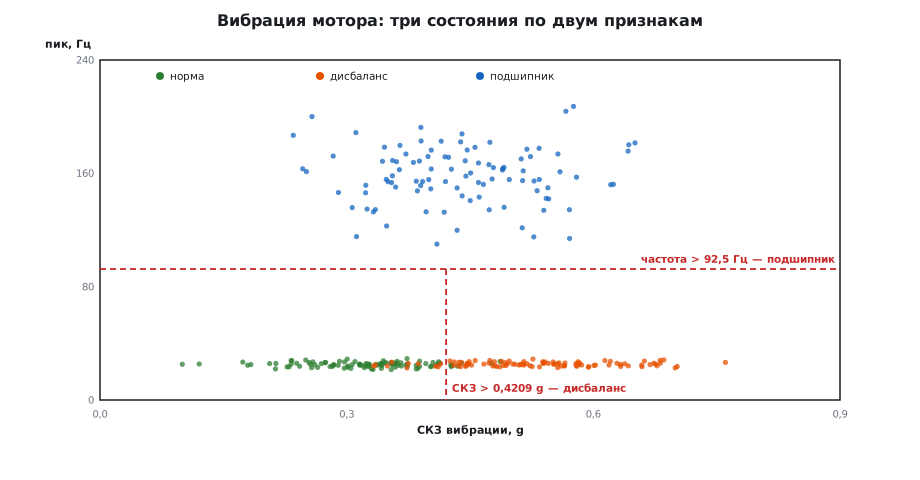
Two features: the RMS vibration, g, and the frequency of the spectral peak, Hz. Three classes: normal, imbalance — a peak at the rotation frequency of 25 Hz with vibration stronger than normal — and bearing wear, with a peak around 160 Hz. The data are synthetic, with a fixed seed: 600 examples for training and 300 for testing, one third per class. Normal and imbalance overlap in RMS, so all five approaches will make mistakes; the question is how many.
116.2 Threshold: two comparisons
int rule_predict(const float x[2])
{
    if (x[1] > F_CUT)
        return 2;
    return x[0] > R_CUT ? 1 : 0;
}
A peak frequency above 92.5 Hz means the bearing; otherwise an RMS above 0.4209 g means imbalance. The RMS threshold is the midpoint between the means of normal and imbalance on the training set. The rule is right in 282 cases out of 300 — better than all the other approaches — stores 2 numbers and does not multiply even once.
116.3 Logistic regression
int logreg_predict(const float x[2])
{
    float z[2], s[3];
    standardize(x, z);
    for (int c = 0; c < 3; c++)
        s[c] = LR_W[c * 2] * z[0] + LR_W[c * 2 + 1] * z[1] + LR_B[c];
    return argmax3(s);
}
Each class gets a weighted sum of the features, and the answer is the largest one. The features are first brought to one scale: otherwise a frequency of hundreds of hertz would swamp an RMS of fractions of a g. 13 numbers, 6 multiplications, 281 correct answers out of 300.
116.4 Decision tree
int tree_predict(const float x[2])
{
    int n = 0;
    while (TREE_LEFT[n] >= 0)
        n = x[TREE_FEAT[n]] <= TREE_THR[n] ? TREE_LEFT[n] : TREE_RIGHT[n];
    return TREE_CLASS[n];
}
A tree of depth 3 has 9 nodes: no more than three comparisons, not a single multiplication. The threshold from 116.2 is the same kind of tree, only built by hand. The trained tree is right in 279 cases out of 300: it fitted its thresholds to the training set a little more closely than it should.
116.5 k nearest neighbours
k-NN does not train at all: it remembers the whole training set and answers by a vote of the five closest examples. Hence the cost — 1204 numbers in memory and 1200 multiplications for every answer, while correct answers are 278 out of 300.
    for (int i = 0; i < N_TRAIN; i++) {
        float dx = z[0] - KNN_X[2 * i], dy = z[1] - KNN_X[2 * i + 1];
        float d = dx * dx + dy * dy;
116.6 A small neural network
A 2 → 8 → 3 perceptron: a hidden layer of 8 neurons with ReLU, and an output layer.
    for (int j = 0; j < N_HIDDEN; j++) {
        float a = MLP_B1[j] + z[0] * MLP_W1[j] + z[1] * MLP_W1[N_HIDDEN + j];
        h[j] = a > 0 ? a : 0;
    }
55 numbers, 40 multiplications, 281 correct answers out of 300 — the same as logistic regression. A neural network wins when the boundary between classes is curved and there are many features; here the boundary is two straight lines, and the network has nothing to add.
116.7 Where they go wrong: the confusion matrix
A single number "right out of 300" hides the main thing — which classes the model confuses. A confusion matrix sorts the answers into pairs "what it was — what the model said". Here all five approaches show the same picture: all five recognize the bearing in 100 cases out of 100 — the peak frequency gives it away — and all the errors fall on the pair "normal — imbalance", which overlap in RMS.
| Approach | Normal taken for imbalance | Imbalance taken for normal |
|---|---|---|
| Threshold | 8 | 10 |
| Logistic regression | 11 | 8 |
| Tree of depth 3 | 2 | 19 |
| k nearest | 10 | 12 |
| Perceptron | 11 | 8 |
The tree errs asymmetrically: it almost never raises a false alarm, but it misses 19 imbalances out of 100. For a device these are different errors: a false alarm costs a call-out of a technician, a missed imbalance costs a bearing a month later. Which error to tolerate is decided by the task, not by accuracy; the threshold is shifted in the needed direction.
116.8 Cross-validation: the difference is within chance
The test set is one of many possible ones, and 282 against 278 may turn out to be luck. Cross-validation splits the training set into 5 parts of 120 examples, tests on each in turn and trains on the rest. The total over the five parts: regression — 547 out of 600, k nearest and the perceptron — 546 each, the tree and the threshold — 541 each. And within one model the accuracy wanders from part to part: for regression from 105 to 113 out of 120. The difference between the approaches on the test set is from 1 to 4 examples out of 300, that is, less than this spread. The honest conclusion: on this task all five approaches are equal, and you choose by cost, not by accuracy.
116.9 How much data you need
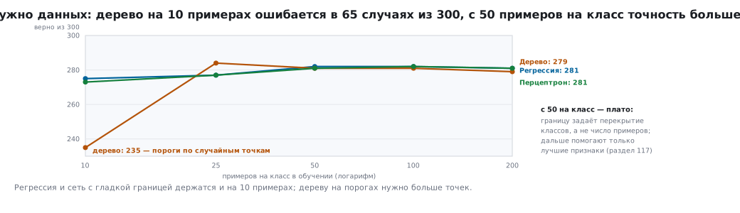
The same models trained on the first 10, 25, 50, 100 and 200 examples of each class, and the same test set of 300:
| Examples per class | Regression | Tree | Perceptron |
|---|---|---|---|
| 10 | 275 | 235 | 273 |
| 25 | 277 | 284 | 277 |
| 50 | 282 | 281 | 281 |
| 100 | 282 | 281 | 282 |
| 200 | 281 | 279 | 281 |
On 10 examples the tree places its thresholds on random points and is wrong in 65 cases, while regression and the network, whose boundary is smooth, hold up. From 50 examples per class the accuracy no longer grows: the boundary between normal and imbalance is set by the overlap of the classes, not by the number of examples. More data helps until the model hits the limits of the data itself; after that only better features help — section 117.
116.10 Comparison table
| Approach | Right out of 300 | Parameters | Multiplications | Code on F407 |
|---|---|---|---|---|
| Threshold | 282 | 2 | 0 | 48 bytes |
| Logistic regression | 281 | 13 | 6 | 176 bytes |
| Tree of depth 3 | 279 | 9 nodes | 0 | 88 bytes |
| k nearest, k = 5 | 278 | 1204 | 1200 | 808 bytes |
| Perceptron 2 → 8 → 3 | 281 | 55 | 40 | 760 bytes |
The answers of the C functions matched the answers of scikit-learn in all 300 cases for each of the five models. Start the choice with a threshold or a tree: they are understandable, you can check them by eye, and they cost almost nothing. Move to a neural network when there are many features and no simple boundary can be found. k-NN on a microcontroller is almost always a bad choice: memory and time grow together with the training set.
116.11 Pitfalls
Accuracy on the training set is 100 %, on the test set it is worse than the threshold. The model memorized the training examples. Accuracy is measured only on data the model has not seen.
The model on the board answers differently from the one on the PC. The features are not brought to the training scale: the mean and the spread must be carried into the firmware together with the weights.
k-NN does not fit in RAM. It stores the whole training set.
The neural network is "better", but makes mistakes in the field. Synthetic and lab data do not look like a real motor; collect data from the object first (section 117).
116.12 Summary
- Five approaches on one task: the threshold — 282 correct out of 300, regression and the perceptron — 281, the tree — 279, k-NN — 278.
- All errors are the pair "normal — imbalance"; the bearing is recognized in 100 cases out of 100. The tree misses 19 imbalances out of 100.
- Cross-validation: the spread from part to part is larger than the difference between the approaches — choose by cost.
- From 50 examples per class accuracy does not grow; on 10 the tree drops to 235.
- The cost differs by orders of magnitude: the threshold is 2 numbers and 48 bytes of code, k-NN is 1204 numbers and 1200 multiplications per answer.
- Start with a threshold and a tree, a neural network — when there are many features.
- The mean and spread of the features are part of the model.
Full sources
infer116.c — inference of five models in C, in float, with parameters from model116.h.
/* Раздел 116: пять моделей — одна задача, вывод на Cortex-M4F во float.
 * Параметры — из model116.h (выгрузил train116.py). На плате каждая функция
 * берёт два признака — СКЗ, g, и частоту пика, Гц — и отвечает классом:
 * 0 — норма, 1 — дисбаланс, 2 — подшипник. На компьютере main сверяет
 * ответы с scikit-learn на проверочной выборке (-DML_HOST).
 * Проверка — _verify/ml116_check.py. */
#include <stdint.h>

#include "model116.h"

/* 1. Порог: два сравнения, ни одного умножения */
int rule_predict(const float x[2])
{
    if (x[1] > F_CUT)
        return 2;
    return x[0] > R_CUT ? 1 : 0;
}

static void standardize(const float x[2], float z[2])
{
    z[0] = (x[0] - MU[0]) / SD[0];
    z[1] = (x[1] - MU[1]) / SD[1];
}

static int argmax3(const float s[3])
{
    int k = 0;
    for (int i = 1; i < 3; i++)
        if (s[i] > s[k])
            k = i;
    return k;
}

/* 2. Логистическая регрессия: три взвешенные суммы, класс — наибольшая */
int logreg_predict(const float x[2])
{
    float z[2], s[3];
    standardize(x, z);
    for (int c = 0; c < 3; c++)
        s[c] = LR_W[c * 2] * z[0] + LR_W[c * 2 + 1] * z[1] + LR_B[c];
    return argmax3(s);
}

/* 3. Дерево решений: спуск по узлам, одно сравнение на уровень */
int tree_predict(const float x[2])
{
    int n = 0;
    while (TREE_LEFT[n] >= 0)
        n = x[TREE_FEAT[n]] <= TREE_THR[n] ? TREE_LEFT[n] : TREE_RIGHT[n];
    return TREE_CLASS[n];
}

/* 4. k ближайших соседей, k = 5: расстояние до каждого обучающего примера */
int knn_predict(const float x[2])
{
    float z[2], best_d[5];
    int best_y[5];
    standardize(x, z);
    for (int i = 0; i < 5; i++) {
        best_d[i] = 3.4e38f;
        best_y[i] = 0;
    }
    for (int i = 0; i < N_TRAIN; i++) {
        float dx = z[0] - KNN_X[2 * i], dy = z[1] - KNN_X[2 * i + 1];
        float d = dx * dx + dy * dy;
        if (d >= best_d[4])
            continue;
        int j = 4;                      /* вставка в отсортированные пять лучших */
        while (j > 0 && best_d[j - 1] > d) {
            best_d[j] = best_d[j - 1];
            best_y[j] = best_y[j - 1];
            j--;
        }
        best_d[j] = d;
        best_y[j] = KNN_Y[i];
    }
    float votes[3] = { 0, 0, 0 };
    for (int i = 0; i < 5; i++)
        votes[best_y[i]] += 1.0f;
    return argmax3(votes);
}

/* 5. Перцептрон 2 → 8 → 3: скрытый слой с ReLU и выходной слой */
int mlp_predict(const float x[2])
{
    float z[2], h[N_HIDDEN], s[3];
    standardize(x, z);
    for (int j = 0; j < N_HIDDEN; j++) {
        float a = MLP_B1[j] + z[0] * MLP_W1[j] + z[1] * MLP_W1[N_HIDDEN + j];
        h[j] = a > 0 ? a : 0;
    }
    for (int c = 0; c < 3; c++) {
        float a = MLP_B2[c];
        for (int j = 0; j < N_HIDDEN; j++)
            a += h[j] * MLP_W2[j * 3 + c];
        s[c] = a;
    }
    return argmax3(s);
}

#ifdef ML_HOST
#include <stdio.h>

int main(void)
{
    static const struct {
        const char *name;
        int (*fn)(const float *);
        const unsigned char *sk;
    } m[5] = {
        { "rule", rule_predict, SK_RULE }, { "logreg", logreg_predict, SK_LOGREG },
        { "tree", tree_predict, SK_TREE }, { "knn", knn_predict, SK_KNN }, { "mlp", mlp_predict, SK_MLP },
    };
    for (int k = 0; k < 5; k++) {
        int same = 0, right = 0;
        for (int i = 0; i < N_TEST; i++) {
            int p = m[k].fn(&TEST_X[2 * i]);
            same += p == m[k].sk[i];
            right += p == TEST_Y[i];
        }
        printf("c_%s=%d,%d\n", m[k].name, same, right);
    }
    printf("done=1\n");
    return 0;
}
#endif
Next: section 117 "Data from the sensor: windows, features, CMSIS-DSP" — where the RMS and the peak frequency come from.