 Embedded HandbookApps
36и. Your own differential probe: isolated amplifier, isolated power, divider and verification
In 36з the differential probe was a finished instrument: two divider arms, a subtractor and a datasheet that states the bandwidth, the common-mode rejection and the category. Here you build it yourself — the way readers discussed it: a signal in a mains circuit up to about a hundred kilohertz, parts for roughly 500 rubles. Instead of two precise arms, this design relies on an isolated amplifier — a chip whose input and output are separated by an isolation barrier, like an optocoupler, but which passes an analog voltage rather than "yes/no". The barrier takes the whole common-mode voltage: the input of the amplifier sits at mains potential, the output at oscilloscope ground.
A few terms you will need below. The hot side is everything before the barrier: the divider or shunt, the amplifier input and its supply; it lives at the potential of the circuit under test. The cold side is everything after the barrier: the amplifier output, the output stage, the cable, the oscilloscope; it is tied to protective earth PE. Isolated power is a small converter with a transformer inside (54.4) that carries energy to the hot side across the same barrier. A shunt is a resistor of a few milliohms on which a current produces a voltage. Input bias current is the current that a chip pin draws from the external circuit by itself, even when there is no signal.
Sources: the 1:10 probe and its compensation — 36а.2; oscilloscope ground — 36а.5
and 36з.1; a floating input and its capacitance to earth — 36з.3; two probes A − B —
36з.5; the differential probe and its arms — 36з.6; CAT categories —
36з.7; cursors — 36е; clearance and creepage — 208.3; the bench for a mains-powered
device — 208.7; isolated power — 54.4; barrier capacitance — 54.5;
the difference amplifier on four resistors — 56.5. The isolated
amplifier is the Novosense NSI1300, datasheet DOC059820010.pdf revision 1.4
(numbers are PDF pages): p. 1 (overview), p. 4 (recommended operating conditions:
input ranges, input common mode, supply), pp. 5–6 (the D05 version), pp. 7–8
(the D25 version), pp. 12–14 (insulation, barrier capacitance, internals), p. 16
(shunt, input filter, output load). The author's oscilloscope is a RIGOL
DHO900: the user guide DHO900_UserGuide_EN.pdf — p. 17 (the probe ground
lead), p. 57 (20 MHz bandwidth limit), p. 58 (1 MΩ input), p. 60
(probe ratios), p. 61 (units and Bias), p. 62 (Ch-Ch Skew);
the datasheet dho900-datasheet.pdf — p. 10 (channel input), p. 19 (Bode
Plot), p. 26 (which models have the generator and Bode Plot). The numbers
in this section are ngspice models and calculations in the stm-lab:1 container
(_verify/probe36i/run36i.sh). There are no datasheets in the project for the voltage isolated amplifier
(NSI1311, NSI1312) or for the isolated DC/DC: they are
described only in general terms, and no numbers are given for them.
What the documentation calls it
Original Meaning isolated amplifier input and output separated by a barrier shunt resistor, Kelvin connection the shunt and its separate sense wires linear full-scale range (FSR), clipping the linear input range and the level where the output saturates input bias current (IIB) the pin current at zero signal single-ended / differential input resistance resistance of one pin / between the pins common-mode output voltage the midpoint around which OUTP and OUTN swing fail-safe output a flag for lost supply or input overload isolation capacitance (CIO) capacitance across the barrier maximum working isolation voltage (VIOWM) the voltage the barrier can hold for its whole life maximum transient isolation voltage (VIOTM) the short-term test voltage common-mode transient immunity (CMTI) tolerance to a fast common-mode jump creepage, clearance distance along the surface, distance through air voltage coefficient of resistance (VCR) resistance drift with the applied voltage compensated divider R and C divide by the same ratio
36и.1 Why build your own and when to buy one
A factory differential probe for hundreds of volts costs as much as a mid-range oscilloscope, yet you need it once a month to look at a triac gate pulse or a heater current. Readers did the math differently: an isolated amplifier in an SOP8 package, a small isolated DC/DC of 1 W, a dozen resistors and an op-amp — about 500 rubles. For signals up to a hundred kilohertz in mains circuits (phase control, zero-cross detector, load current, a slow power factor corrector) this is enough: in the model of the whole chain (36и.6) the −3 dB bandwidth is 269.8 kHz, and at 100 kHz the loss is only −0.30 dB.
What such a probe cannot do — and when you buy one instead of building it:
- fast edges. The 10–90 % rise time of the whole chain in the model is 1.45 µs, the delay is 1.74 µs. A MOSFET switches in tens of nanoseconds: a home-made probe shows that edge smeared a thousand times;
- common-mode rejection at megahertz. The barrier passes the current of its capacitance (36и.7), and every fast common-mode edge shows up as spikes on the screen — for a factory probe this is measured and stated in the datasheet;
- category. A home-made probe has no CAT category at all (36и.10). Where CAT II or higher marking is needed — a distribution board, a service entrance, field work — only a factory probe with a datasheet;
- several channels with identical parameters and measurements on which decisions are made (acceptance, certification) — also a factory probe.
36и.2 How it works: divider, barrier, power, output stage
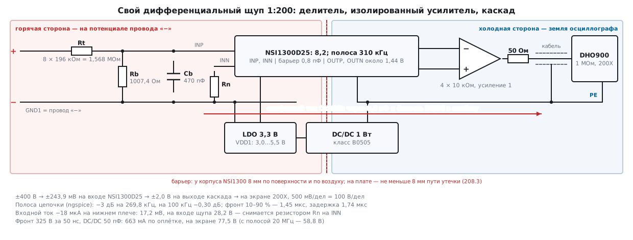
The chain has four parts (figure below):
- Input. For voltage — a divider: an upper arm made of a string of resistors totalling megohms and a lower arm of about a kilohm. For current — a shunt. The input of the isolated amplifier gets fractions of a volt.
- The isolated amplifier NSI1300. The input is differential, INP and INN, relative to its own ground GND1 (the hot side). Inside is a sigma-delta modulator: it turns the input into a bit stream, the stream crosses the capacitive barrier, and on the cold side a 4th-order filter turns it back into a voltage (p. 14). The output is also differential: OUTP and OUTN swing around 1.44 V (p. 6).
- Isolated power for the hot side. The amplifier input is powered from VDD1 relative to GND1 — from 3.0 to 5.5 V (p. 4). This supply is taken from the cold side through an isolated DC/DC of the "B0505" class (5 V to 5 V, 1 W): the hot side draws 11.4 mA typical and 15.1 mA maximum (pp. 5 and 7), that is 57.0–75.5 mW, 5.7–7.5 % of a module rated 1 W. An unregulated module at such a light load raises its output above nominal (54.4) — by how much, only its datasheet will say — so it is followed by a 3.3 V LDO regulator.
- Output stage. A difference amplifier on an op-amp and four resistors (56.5) turns the difference OUTP − OUTN into one voltage relative to the cold-side ground, and through a 50 Ω resistor and a coaxial cable it goes to the oscilloscope input.
The key design decision: the hot-side GND1 is the "−" lead of the probe itself. The common-mode voltage passes through no divider: the whole hot side "rides" along with the "−" lead, and the divider divides only the difference between "+" and "−". That has a price: the "−" lead is a direct connection to the hot-side electronics, with no resistance of megohms, and it must be insulated like a mains wire (36и.10).
The scale is chosen so that the screen gets a standard probe ratio. The gain of the NSI1300D25 is 8.2, the stage is 1; a 1:1640 divider gives exactly 1:200 together. An input of ±400 V becomes ±243.9 mV at the amplifier input (the linear range is ±250 mV) and ±2.0 V at the output of the stage. The DHO900 probe menu has the ratio 200X (user guide, p. 60): at 500 mV/div the screen shows 100 V/div, and ±400 V fill all 8 divisions.
36и.3 Current probe: a shunt at the NSI1300 input
Current is what the NSI1300 was made for: the datasheet states its purpose directly — shunt-based current sensing in high-voltage circuits (pp. 1 and 16). It comes in two versions, which differ in input range:
| Version | Linear input | Before clipping | Gain | Input R (INN at GND1 / between inputs) | Input bias current | Offset |
|---|---|---|---|---|---|---|
| NSI1300D25 | ±250 mV | ±320 mV | 8.2 | 19 kΩ / 22 kΩ | −18 µA (−24…−12) | ±0.2 mV max |
| NSI1300D05 | ±50 mV | ±64 mV | 41 | 4.75 kΩ / 4.9 kΩ | −22 µA (−29…−14) | ±0.1 mV max |
(datasheet, pp. 4, 5 and 7). The minus sign of the bias current means that the current flows out of the pin into the external circuit.
The rule for choosing the shunt is in the datasheet (p. 16): at the rated current the drop is no more than the linear range, at the maximum allowed current — no more than the clipping level. Example — the 2000 W heater from 36з.8: 8.70 A rms, 12.30 A at the sine peak.
| NSI1300D25 | NSI1300D05 | |
|---|---|---|
| shunt at most | 20.3 mΩ → take 20 mΩ | 4.1 mΩ → take 4 mΩ |
| drop at the 12.30 A peak | 246.0 mV | 49.2 mV |
| output clips at | 16.0 A | 16.0 A |
| shunt power at 8.70 A | 1.51 W | 0.30 W |
| offset ±0.2 / ±0.1 mV in amperes | ±10 mA | ±25 mA |
| two 10 Ω filter resistors at the input | −0.09 % | −0.41 % |
What follows from this:
- Power versus accuracy. The D05 heats the shunt five times less (0.30 W versus 1.51 W), but its offset converted to current is larger: ±25 mA versus ±10 mA. A shunt dissipating 1.51 W is chosen with a twofold power margin, and you make sure its heating does not shift its resistance — the shunt's drift with temperature is not covered by the amplifier datasheet.
- The input filter loads the input. The datasheet recommends an RC filter between the shunt and the input (p. 16). Two 10 Ω resistors against the input resistance between the pins give a gain error: for the D25 (22 kΩ) −0.09 %, for the D05 (4.9 kΩ) already −0.41 % — more than the chip's own gain error of ±0.3 % (p. 5). The filter resistors are kept as small as possible and equal.
- Bias current through the filter resistors. 18 µA through 10 Ω is 0.18 mV on each pin, for the D05 22 µA gives 0.22 mV: as much as the maximum offset of the chip itself. With equal resistors on both inputs these voltages subtract; how precisely depends on the difference between the two pin currents, which the datasheet does not specify. The rest is removed by zero calibration (36и.9).
- Kelvin connection (p. 16): a separate twisted, symmetrical pair of sense wires to the shunt, not the same traces that carry the current. The shunt sits in the mains circuit, so GND1 is at one of its ends, and the whole hot side is at mains potential.
Scale on the screen: 20 mΩ × 8.2 — 0.164 V/A at the amplifier output. To get a round 0.1 V/A, the stage gets a gain of 0.6098: resistors of 6.09 kΩ over 10 kΩ give 0.0999 V/A. On the DHO900 set the channel unit to A (user guide, p. 61) and the ratio to 10X (p. 60) — the screen shows amperes.
36и.4 Voltage probe: a divider at the NSI1300 input
a) A divider on the NSI1300 — an honest calculation
The NSI1300 is designed for a shunt of milliohms. A divider of megohms is a completely different source, and two properties of the chip input that go unnoticed on a shunt show up: the input resistance loads the lower arm, and the bias current flowing through the lower arm creates an offset.
First — which numbers to take. The discussion mentioned 4.9 kΩ and −22 µA; according to the datasheet this is the D05 version (±50 mV, gain 41, p. 5). For ±250 mV it is the D25 version: 22 kΩ between the pins, 19 kΩ from INP to GND1 with INN at GND1, bias current −18 µA (p. 7). In the divider INN sits on GND1, so it is the 19 kΩ that loads the lower arm.
The input model (div36i.cir) is what the datasheet gives as numbers: a resistor
from the pin to GND1 and a current source flowing out of the pin:
.subckt nsi pin rin=19k ib=18u
Rin pin 0 {rin}
Ib 0 pin {ib}
.ends
The upper arm is 8 × 196 kΩ = 1.568 MΩ (why eight — 36и.5). The lower arm together with the input must give 1:1640: 956.68 Ω, so the lower-arm resistor is 1007.4 Ω (in practice 910 Ω and a 200 Ω trimmer — adjustment is needed anyway, 36и.9). The two versions compared at the same 1:200 on the screen:
| D25 (±250 mV) | D05 (±50 mV) | |
|---|---|---|
| divider | 1:1640 | 1:8200 |
| 400 V at the amplifier input | 243.9 mV | 48.8 mV |
| lower arm together with the input | 956.68 Ω | 191.24 Ω |
| lower-arm resistor | 1007.4 Ω | 199.3 Ω |
| offset from the bias current | 17.2 mV — 7.1 % of scale | 4.21 mV — 8.6 % of scale |
| the same at the probe input | 28.2 V | 34.5 V |
| output noise (100 kHz bandwidth) → at the probe input | 195 µV → 39 mV | 260 µV → 52 mV |
| chip offset drift → at the probe input | up to 6.6 mV/°C | up to 8.2 mV/°C |
The ngspice model with the D25 shows what this means in volts:
- with zero at the probe input the amplifier input already has 17.2 mV — the screen shows 28.2 V where zero should be;
- at +400 V the amplifier input gets 261.1 mV — beyond the linear range of ±250 mV, although the divider itself is designed for 243.9 mV; at −400 V — −226.7 mV. The offset ate the headroom on one side;
- the bias current varies between parts from −12 to −24 µA (p. 7): an offset from 11.5 to 22.9 mV, from 18.8 to 37.6 V at the probe input. Every probe you build needs its own zero calibration;
- the input resistance is given only as a typical value. If a part has it 20 % lower or higher, the divider ratio shifts by −1.24 % or +0.85 %: ratio adjustment is also per part.
The cure for the offset is a resistor Rn on INN. The same resistor as the lower arm, between INN and GND1: the INN bias current creates the same offset on it, and it subtracts in the difference. In the model with Rn the zero is −0.01 mV, and +400 V gives exactly 243.9 mV. What remains depends on the difference between the bias currents of the two pins, which the datasheet does not specify: each microampere of difference is 0.957 mV at the amplifier input, 1.57 V at the probe input. Zero calibration removes it.
Checking the input common mode: the amplifier input works only while the average of INP and INN relative to GND1 stays between −160 and +800 mV (p. 4). At −400 V at the probe input it is −113 mV — inside. Drift: the chip offset up to 4 µV/°C (p. 7) is 6.6 mV/°C at the probe input, the drift of the bias current on the lower arm is 1.57 mV/°C; over 30 °C of warm-up — 0.24 V. For a probe whose full scale is 400 V this is tolerable, but the zero is checked after warm-up.
b) Why a voltage amplifier with a high-impedance input is better
The same manufacturer makes isolated amplifiers designed specifically for a voltage divider — NSI1311 and NSI1312 ("voltage sensing" class). Their datasheets are not in the project, so here is only the principle, without numbers. Such an amplifier has a high-impedance input and a small bias current: the lower arm of the divider can be tens of kilohms rather than one kilohm, and neither the input resistance nor the bias current affects it noticeably. Then the upper arm is tens of megohms too, and it heats less. For example, if the input allows a 10 kΩ lower arm, then at the same 1:1640 the upper one is 16.4 MΩ, and at 400 V it dissipates 9.8 mW instead of 102 mW (36и.5). What exactly the input allows — range, input resistance, bias current, common mode — is in the datasheet of the specific chip.
36и.5 Divider: voltage, power, voltage coefficient, compensation
Why a string and not one resistor. Every resistor has a maximum working voltage and a maximum pulse — per its datasheet (not in the project). The upper arm is split into several identical resistors so that each gets less. For 8 × 196 kΩ:
- at 400 V — 102 mW for the whole arm, 50 V and 12.7 mW on each resistor;
- at 230 V rms mains — 33.7 mW for the arm;
- at a 2500 V surge — a typical value for equipment plugged into an outlet (208.3) — each resistor gets 312.5 V, and the current into the amplifier pin is 1.59 mA. The pin withstands 10 mA through its protection diodes (p. 14), but whether the resistors themselves survive 312.5 V depends on their datasheet; for pulses there are special high-voltage and pulse-rated resistors.
Millimetres. The string is laid out in a line with gaps: between neighbouring resistors the difference is 50 V, but between the first and the last — all 400. Between the hot and cold sides reinforced insulation is needed: creepage of about 8 mm (208.3, 54.5), a strip free of copper on all layers, a slot under the package if the millimetres are not enough. The NSI1300 package gives 8 mm both along the surface and through air (p. 12) — the board under it must not shorten that path.
Voltage coefficient. The resistance of a thick-film resistor depends slightly on the applied voltage. The number is in the resistor datasheet; the calculation uses two assumptions, 10 and 50 ppm/V. The divider ratio shift at 400 V:
| Resistors in the arm | On each | At 10 ppm/V | At 50 ppm/V |
|---|---|---|---|
| 2 | 200 V | 0.20 % | 1.00 % |
| 4 | 100 V | 0.10 % | 0.50 % |
| 8 | 50 V | 0.05 % | 0.25 % |
This shift grows with voltage, so it produces nonlinearity: a calibration at 30 V will not reveal it. The more resistors in the string, the less voltage on each and the smaller the shift. The lower arm sees less than 0.25 V — its voltage coefficient does not matter.
Compensation. Like a 1:10 probe (36а.2), the divider has two "branches": the resistors and the stray capacitances. The capacitance of the upper arm is a fraction of a picofarad (in the model, an assumption of 0.1 pF for the whole arm), the time constant Rt·Ct = 156.8 ns. For exact compensation the lower arm needs 163.9 pF, and without a capacitor it has only the amplifier input of 2 pF (p. 5) and the wiring (an assumption of 5 pF). How much the divider passes at high frequencies relative to DC, for different upper-arm capacitances:
| Upper-arm capacitance | Cb 7 pF (no capacitor) | Cb 157 pF | Cb 477 pF |
|---|---|---|---|
| 0.05 pF | 11.63 | 0.52 | 0.17 |
| 0.10 pF | 23.10 | 1.04 | 0.34 |
| 0.20 pF | 45.56 | 2.09 | 0.69 |
| 0.30 pF | 67.40 | 3.13 | 1.03 |
The ngspice model (div36i.cir, upper arm 0.1 pF): without a capacitor the divider
starts to pass more than it should from 1.01 MHz (+3 dB), and at 100 MHz —
22.5 times more. With 157 pF it is almost flat: +4.4 % at 100 MHz.
With 477 pF it is already a filter: −3 dB at 398 kHz, at 100 kHz — 0.966.
The choice for a home-made probe is the third column. You cannot tune 157 pF to an unknown 0.1 pF: the upper-arm capacitance depends on the layout, the wires, a hand nearby, and at 0.2 pF instead of 0.1 the same capacitor already gives a twofold overshoot. With 470 pF the lower arm "leads": for any upper-arm capacitance from 0.05 to 0.3 pF high frequencies do not pass more strongly than DC. This is exactly the input RC filter that the datasheet recommends before the input (p. 16) — the modulator does not receive high-frequency interference that it could shift down in frequency.
36и.6 Bandwidth and rise time of the whole chain
The chain: divider → NSI1300D25 → difference stage → 50 Ω and cable →
DHO900 input 1 MΩ ‖ 15 pF (DHO900 datasheet, p. 10). The NSI1300 bandwidth is
310 kHz typical, 250 kHz minimum; the output rise time is 1.3 µs, the delay
from input to output is 1.6 µs typical and 2.1 µs maximum (pp. 6 and 8).
The datasheet does not name the type of the 4th-order output filter, so
the model (chain36i.cir) has two variants: Butterworth (flat frequency response,
has overshoot) and Bessel (no overshoot, rolls off earlier). The stage op-amp has
a gain-bandwidth product of 10 MHz (assumption), the 1 m cable is
100 pF (assumption).
| Filter in the model | Cb | −3 dB | At 100 kHz | Rise 10–90 % | Delay | Overshoot |
|---|---|---|---|---|---|---|
| Butterworth | 150 pF | 309.8 kHz | 0.00 dB | 1.25 µs | 1.48 µs | 10.9 % |
| Butterworth | 470 pF | 269.8 kHz | −0.30 dB | 1.45 µs | 1.74 µs | 6.4 % |
| Bessel | 150 pF | 307.6 kHz | −0.29 dB | 1.14 µs | 1.10 µs | 0.8 % |
| Bessel | 470 pF | 230.9 kHz | −0.60 dB | 1.48 µs | 1.37 µs | none |
What this shows. The bandwidth is set by the amplifier: the stage, the 50 Ω and the cable mean nothing at hundreds of kilohertz (the ratio at 1 kHz differs from 1:200 by −0.01 %). With the 150 pF divider the Butterworth model is closer to the datasheet — rise time 1.25 µs versus 1.3 µs, delay 1.48 µs versus 1.6 µs (the rest is the delay of the modulator itself, which the model does not know) — but whether the real chip has an overshoot of 10.9 %, the datasheet does not say. This is checked with a square wave (36и.9). With 470 pF the bandwidth drops to 230.9–269.8 kHz, but the hundred kilohertz the probe was built for passes with a loss of 0.30–0.60 dB.
Delay — a pitfall when comparing channels. The signal through the probe lags by 1.6–2.1 µs behind a channel connected directly. The Ch-Ch Skew adjustment on the DHO900 is from −100 to +100 ns (user guide, p. 62), the probe delay is 16–21 times larger. Measure it with cursors (36е) on a common signal and subtract it mentally, or view all the signals being compared through identical probes.
36и.7 Barrier capacitance and common-mode current
Galvanically the barrier breaks the circuit, but the capacitance between the sides
remains (54.5): for the NSI1300 it is 0.8 pF (p. 13), for an isolated DC/DC it is
the transformer windings, tens of picofarads (54.5); there is no exact number for
a specific module in the project. When the "−" lead jumps together
with the measured point, a current i = C·dV/dt flows through these capacitances — this is
the same story as in 36з.3 with the battery-powered oscilloscope, except the current
flows not through the ground clip but across the barrier into the cable shield and on into PE.
First — the amplifier itself. Its common-mode transient immunity is 150 kV/µs typical, 100 kV/µs minimum (pp. 6 and 8). An edge of 325 V in 1 µs (a triac) is 0.325 kV/µs, in 50 ns (a MOSFET) — 6.500 kV/µs: a margin of 23.1 times (15.4 at the minimum). For silicon carbide and gallium nitride switches, where edges are several times steeper, this margin is recalculated.
Current across the barrier (total capacitance — 0.8 pF of the amplifier plus the DC/DC):
| DC/DC capacitance (assumption) | Current, 1 µs edge | On screen, 1 µs: full bandwidth / 20 MHz | Peak current, 50 ns edge | On screen, 50 ns: full bandwidth / 20 MHz |
|---|---|---|---|---|
| 2 pF | 0.92 mA | 1.41 / 0.37 V | 40 mA | 29.5 / 7.5 V |
| 10 pF | 3.54 mA | 1.50 / 0.83 V | 143 mA | 41.8 / 19.9 V |
| 50 pF | 17.0 mA | 4.25 / 3.44 V | 663 mA | 77.5 / 58.8 V |
The model (cm36i.cir): both probe leads on one point that jumps
by 325 V, the correct answer is 0. The "−" lead is 15 cm, like the ground clip in 36з.
The cold side goes to oscilloscope ground through the shield of a 1 m cable,
whose inductance, resistance and coupling to the centre conductor are
model assumptions. Errors are referred to the probe input (× 200).
Three conclusions:
- The amplifier itself is clean. At its input on a 50 ns edge there is up to 2.33 V referred to the probe input (the drop on the "−" lead, as in 36з.3), but after its 310 kHz filter no more than 1.9 mV remains at the output: the inductive spike is short, and its average is zero.
- The spikes are drawn by the current return path. The current across the barrier returns through the shield, and the drop on it adds to the signal right at the oscilloscope input — after all the probe filters. Hence the scale: the larger the DC/DC capacitance, the larger the current (40 → 143 → 663 mA peak) and the spike.
- What helps: a DC/DC with a low barrier capacitance (at 2 pF the current is almost four times smaller than at 10 pF); the 20 MHz oscilloscope bandwidth limit (DHO900 user guide, p. 57; datasheet, p. 10) — the useful signal of the probe is below 310 kHz anyway, and the 50 ns spike drops from 29.5 to 7.5 V at 2 pF; a short cable and a ferrite ring on it — the model does not include these.
36и.8 The output stage and the cable to the DHO900
The NSI1300 output is the pair OUTP and OUTN around a common mode of 1.44 V (from 1.39 to 1.49 V, p. 6), output resistance below 0.2 Ω, and the datasheet advises at least 1 kΩ on the pins so as not to overload them (p. 16). A difference stage on four resistors of 10 kΩ does exactly that: its input resistors are the output load, and a gain of 1 turns the difference into one voltage relative to the cold-side ground.
The stage's common-mode rejection is set by the resistors (56.5). The common mode of
1.44 V here is constant, and what remains of it is a zero offset. The model
(out36i.cir), the worst combination of tolerances, as in 56.5:
| Resistor tolerance | At the output from 1.44 V | At the probe input (× 200) | Rejection |
|---|---|---|---|
| 0.1 % | 2.88 mV | 0.58 V | 54.0 dB |
| 1 % | 28.5 mV | 5.70 V | 34.1 dB |
With 0.1 % resistors that is 0.58 V of offset on the ±400 V scale, removed by zero calibration. With 1 % — 5.70 V, and moreover this offset varies with the output common mode from part to part: use 0.1 %.
What the characteristic levels on the screen mean (at 200X):
- the output clips at ±2.45 V (p. 14) — ±490 V on the screen. A flat "shelf" at this level is input overload, not a signal;
- the fail-safe output is −2.5…−2.6 V (p. 6) — −500…−520 V on the screen. The chip produces it when the hot-side supply is lost or the input common mode exceeds 0.9 V (pp. 5 and 14). A probe that "shows −500 V" with no signal is a probe without VDD1: check the DC/DC and the LDO.
Cable and oscilloscope input. The DHO900 has only a 1 MΩ ±1 % and 15 pF ±3 pF input (user guide, p. 58; datasheet, p. 10). The 50 Ω resistor at the op-amp output isolates it from the cable capacitance, and against 1 MΩ it gives an error of 50 ppm. The wavelength in the cable at 310 kHz is 639 m, so cable termination is not needed at these frequencies. The cold-side supply is bipolar ±5 V for the op-amp (output ±2 V) and 3.3 V for VDD2 (from 3.0 to 5.5 V, p. 4).
DHO900 settings. Probe ratio 200X (user guide, p. 60), 500 mV/div — 100 V/div on the screen, ±400 V — all 8 divisions. The remaining zero offset after calibration can be removed with the Bias adjustment in the Vertical menu (p. 61). For the current probe — unit A and 10X (36и.3).
36и.9 Verification and calibration
The order goes from safe to dangerous. Until steps 1–4 are done, the probe sees no mains voltage.
1. No input. With an ohmmeter — check there is no conduction between the hot and cold sides (open on the megohm range). Power the cold side: VDD1 on the hot side must be from 3.0 to 5.5 V. Leads "+" and "−" shorted: the screen shows the offset left after Rn. If instead it shows −500 V — there is no VDD1 (36и.8).
2. DC voltage. From a 30 V lab supply, measured with a multimeter: 0.150 V at the output, 30 V on the screen at 200X. Use the lower-arm trimmer to make them match, then reverse the polarity — check symmetry. Check the zero again after 20–30 minutes of warm-up (36и.4).
3. Frequency response. A generator (36к) — a sine into the probe input, the "−" lead to the generator ground; compare with the same signal fed directly to a second channel. The DHO914S and DHO924S models have a built-in generator and Bode Plot (datasheet, p. 26): from 10 Hz to 25 MHz, amplitude from 20 mV to 5 V (p. 19). 5 V at the probe input is 25 mV at its output, enough for a comparison with the direct channel. Expected from the model: at 100 kHz −0.30…−0.60 dB, −3 dB at 230.9…269.8 kHz. Then a square wave: the overshoot on the edge shows whether the chip filter is closer to Butterworth (6.4 % in the model) or to Bessel (none), and a "droop" or a "hump" after the edge shows under- or overcompensation of the divider (36и.5).
4. Common mode at low voltage. Both probe leads together — on the generator output, the generator ground connected to the oscilloscope ground. Everything visible on the screen is common-mode leakage. On a 50 Hz sine there is almost none; a square wave with steep edges shows the spikes from 36и.7 — their size depends on the DC/DC and the cable. Turn on the 20 MHz bandwidth limit and compare.
5. Mains — only with current limiting. The bench from 208.7: an RCD, an isolation transformer, one hand.
- Differential at mains voltage: the probe on the secondary of an isolation transformer with a lamp or a resistor in series. 230 V rms gives 1.15 V rms at the output, 1.626 V peak.
- Common mode at mains voltage: an isolation transformer does not work here — its secondary is not tied to earth, so there is no common mode relative to the oscilloscope. Both probe leads together through a 100 kΩ resistor to the phase, behind an RCD: at any breakdown the current is no more than 2.3 mA. Only noise should remain on the screen.
- Connect and disconnect the leads with the mains off, the probe and the board on an insulating stand, no hands during the measurement.
36и.10 Safety: what a home-made probe is not
⚠️ A home-made probe is not a CAT II probe. A category means a tested design: clearances, enclosure, leads, impulse withstand, verified against the standard (36з.7). A home-made probe has not had a single one of these tests, so it has no category either — whatever numbers the chip datasheet states.
The limitations that follow:
- The rating of the chain is set by the weakest link (36з.7). The NSI1300 barrier is reinforced, working voltage 1500 V rms (pp. 12 and 14) — 6.5 times the 230 V mains, short-term test voltage 8000 V peak (p. 13). But the DC/DC also crosses the barrier: what insulation it has — functional, basic or reinforced — and for what working voltage, only its datasheet will say. The test voltage of a module ("1.5 kV", "3 kV") is not the working voltage (54.5). The board, the enclosure and the leads are yours, and nobody has tested them.
- The "−" lead is GND1. It is connected directly to the hot side, with no megohms. The leads must be mains-rated test leads with shrouded 4 mm plugs; the hot side in a closed insulating enclosure with no accessible metal parts; connectors and fixings that keep the leads from being pulled out.
- Only the bench from 208.7. The device under test — through an RCD, if possible through an isolation transformer; circuits that plug into an outlet. Never distribution boards, service entrances, breakers (that is CAT III and above, 36з.7).
- The oscilloscope is earthed. The cold side of the probe is tied to PE through the cable shield and the oscilloscope chassis: if the barrier breaks down, the current goes to PE and the protection trips. On the DHO900 PE is connected via the terminal on the rear panel (36з.1); the probe ground lead goes to ground only (user guide, p. 17). Never cut PE off the oscilloscope — without it a broken barrier puts the mains on the chassis, all BNCs and cables.
- The limit is written on the enclosure. A label "not more than 400 V peak, bench 208.7 only, no CAT" — for whoever picks up the probe a year from now.
36и.11 Pitfalls
The screen shows 28 V where zero should be, and +400 V clips before −400. The NSI1300 bias current on the lower arm: 17.2 mV, 28.2 V at the probe input; +400 V gives 261.1 mV — beyond the linear range. A resistor Rn on INN and zero calibration (36и.4).
You took 4.9 kΩ and −22 µA for a ±250 mV divider. These are the numbers of the D05 version (±50 mV). The D25 has 19 kΩ from INP to GND1 and −18 µA (36и.4).
The ratio varies from part to part. The input resistance is given only as typical: ±20 % means −1.24…+0.85 % of the ratio. A trimmer in the lower arm and calibration (36и.9).
A square wave with a hump or a step after the edge. The divider is not compensated; tuning a capacitor to an unknown upper-arm capacitance does not work — a 470 pF lower arm leads (36и.5).
At 400 V the reading "drifts", although at 30 V everything is accurate. The voltage coefficient of the upper-arm resistors: at 50 ppm/V and two resistors — 1.00 %. More resistors in the string (36и.5).
A MOSFET edge on the screen is a gentle slope of one and a half microseconds. That is not the circuit, it is the probe bandwidth: the 10–90 % rise time in the model is 1.25–1.48 µs (36и.6). For nanosecond edges — a factory probe.
The channels "drifted apart" by 1.6 µs, and Skew does not help. Ch-Ch Skew on the DHO900 is ±100 ns; the probe delay is 16–21 times larger (36и.6).
Every switch edge shows a spike of tens of volts. The current through the barrier capacitance and the DC/DC into the shield: 50 pF on a 50 ns edge — 663 mA and 77.5 V. A low-capacitance DC/DC, a 20 MHz bandwidth limit, a short cable (36и.7).
The probe shows −500 V with nothing at the input. The NSI1300 fail-safe output: no hot-side supply or the input common mode above 0.9 V (36и.8).
An offset of 5.7 V that calibration does not remove. Stage resistors of 1 %: 28.5 mV remain from the 1.44 V output common mode. Use 0.1 % resistors (36и.8).
You checked the common mode through an isolation transformer — perfect. The transformer secondary is not tied to earth, there was no common mode. Common mode is checked relative to the oscilloscope ground — through a 100 kΩ resistor to the phase (36и.9).
36и.12 Summary
- Your own differential probe is a divider or shunt, an isolated amplifier across the barrier, isolated power for the hot side and a difference stage to the oscilloscope. GND1 is the "−" lead: the barrier holds the whole common mode.
- The NSI1300 is made for a shunt: D25 for ±250 mV (20 mΩ for 12.30 A, 1.51 W) or D05 for ±50 mV (4 mΩ, 0.30 W, but ±25 mA of offset).
- A divider on the NSI1300D25: 1:1640 and 1:200 on the screen; the 19 kΩ input loads the lower arm, the −18 µA bias current gives 17.2 mV (28.2 V at the probe input) — Rn on INN and zero calibration. The numbers 4.9 kΩ and −22 µA belong to the D05 version. A voltage amplifier with a high-impedance input is more convenient — per its datasheet.
- The upper arm is a string (8 × 196 kΩ: 50 V and 12.7 mW each at 400 V), 8 mm of creepage between the sides, the voltage coefficient gives nonlinearity; a 470 pF lower arm leads, and the compensation does not depend on the unknown upper-arm capacitance.
- The chain bandwidth in the model is 230.9–309.8 kHz, at 100 kHz no worse than −0.60 dB; rise time 1.14–1.48 µs, delay 1.10–1.74 µs — more than the DHO900 Ch-Ch Skew (±100 ns).
- Barrier capacitance: the C·dV/dt current flows into the shield and draws spikes on edges — a low-capacitance DC/DC, a 20 MHz bandwidth limit.
- Stage: 0.1 % resistors (54.0 dB, 0.58 V of offset); −500 V on the screen is the fail-safe output, no VDD1.
- Verification goes from the ohmmeter to the mains: zero, 30 V, frequency response and square wave, common mode from the generator, then mains through a transformer and through 100 kΩ.
- A home-made probe has no category: only the 208.7 bench, the oscilloscope on PE, the limit written on the enclosure.
Full sources
div36i.cir — the divider at the NSI1300 input: loading by the input, bias current, compensation.
* 36и.4, 36и.5: делитель ±400 В на вход NSI1300 — нагрузка входом, входной ток, компенсация.
* Вход NSI1300 по даташиту (RIN при INN = GND1 и IIB при INP = INN = GND1) в модели —
* резистор RIN от вывода к GND1 и источник тока IIB, вытекающий из вывода (IIB < 0).
* D25 (±250 мВ, усиление 8,2): RIN 19 кОм, IIB −18 мкА; D05 (±50 мВ, усиление 41): RIN 4,75 кОм, IIB −22 мкА.
* GND1 — узел 0: это провод «минус» щупа. Верхнее плечо 8 x 196 кОм = 1,568 МОм.
* Нижнее плечо подогнано: 1:1640 для D25 (8,2 x 200), 1:8200 для D05 (41 x 200).
.subckt nsi pin rin=19k ib=18u
Rin pin 0 {rin}
Ib 0 pin {ib}
.ends
Vp p 0 DC 0
* 1: D25, INN прямо на GND1
Rt1 p a1 1.568meg
Rb1 a1 0 1007.4
X1 a1 nsi
* 2: D25, на INN резистор Rn = Rb: входной ток INN даёт такое же смещение
Rt2 p a2 1.568meg
Rb2 a2 0 1007.4
X2 a2 nsi
Rn2 n2 0 1007.4
X2n n2 nsi
* 3: D05, INN прямо на GND1
Rt3 p a3 1.568meg
Rb3 a3 0 199.3
X3 a3 nsi rin=4.75k ib=22u
* 4, 5: D25 с RIN на 20 % меньше и больше типового (в даташите только типовое)
Rt4 p a4 1.568meg
Rb4 a4 0 1007.4
X4 a4 nsi rin=15.2k
Rt5 p a5 1.568meg
Rb5 a5 0 1007.4
X5 a5 nsi rin=22.8k
* 6: D25, IIB −12 и −24 мкА (мин. и макс. по даташиту)
Rt6 p a6 1.568meg
Rb6 a6 0 1007.4
X6 a6 nsi ib=12u
Rt7 p a7 1.568meg
Rb7 a7 0 1007.4
X7 a7 nsi ib=24u
* компенсация: верх 1,568 МОм || 0,1 пФ (допущение), низ 1007,4 Ом || Cb, вход 19 кОм, 2 пФ вывода + 5 пФ монтажа
Vac q 0 DC 0 AC 1
Rt8 q b1 1.568meg
Ct8 q b1 0.1p
Rb8 b1 0 1007.4
Ri8 b1 0 19k
Cb8 b1 0 7p
Rt9 q b2 1.568meg
Ct9 q b2 0.1p
Rb9 b2 0 1007.4
Ri9 b2 0 19k
Cb9 b2 0 157p
Rt10 q b3 1.568meg
Ct10 q b3 0.1p
Rb10 b3 0 1007.4
Ri10 b3 0 19k
Cb10 b3 0 477p
E8 o1 0 b1 0 1640
E9 o2 0 b2 0 1640
E10 o3 0 b3 0 1640
.control
dc Vp -400 400 400
let d2 = v(a2) - v(n2)
meas dc d25_off FIND v(a1) AT=0
meas dc d25_p400 FIND v(a1) AT=400
meas dc d25_m400 FIND v(a1) AT=-400
meas dc d25n_off FIND d2 AT=0
meas dc d25n_p400 FIND d2 AT=400
meas dc d05_off FIND v(a3) AT=0
meas dc d05_p400 FIND v(a3) AT=400
meas dc rlo_p400 FIND v(a4) AT=400
meas dc rlo_off FIND v(a4) AT=0
meas dc rhi_p400 FIND v(a5) AT=400
meas dc rhi_off FIND v(a5) AT=0
meas dc ib12_off FIND v(a6) AT=0
meas dc ib24_off FIND v(a7) AT=0
ac dec 50 10 300meg
meas ac bare_lf FIND vm(o1) AT=10
meas ac bare_hf FIND vm(o1) AT=100meg
meas ac c157_hf FIND vm(o2) AT=100meg
meas ac c157_100k FIND vm(o2) AT=100k
meas ac c477_100k FIND vm(o3) AT=100k
meas ac c477_f3 WHEN vdb(o3)=-3
meas ac bare_f3up WHEN vdb(o1)=3
.endc
.end
chain36i.cir — frequency response and rise time of the whole 1:200 chain: two filter variants and two lower arms.
* 36и.5, 36и.6: АЧХ и переходная характеристика всей цепочки щупа 1:200.
* Делитель: верх 1,568 МОм (8 x 196 кОм) || 0,1 пФ паразитной ёмкости (допущение),
* низ 1007,4 Ом || Cb, параллельно вход NSI1300D25: 19 кОм и 2 пФ, плюс 5 пФ монтажа (допущение).
* NSI1300D25: усиление 8,2 и фильтр 4-го порядка на 310 кГц; тип фильтра в даташите не указан —
* две модели: Баттерворт (Q 0,5412 и 1,3066) и Бессель (1,4192 fc, Q 0,5219; 1,5912 fc, Q 0,8055).
* Выход: OUTP/OUTN вокруг 1,44 В, ROUT 0,2 Ом. Разностный каскад 10 кОм x 4 на ОУ с GBW 10 МГц
* (допущение), 50 Ом, кабель 100 пФ (1 м, допущение), вход DHO900 1 МОм || 15 пФ.
* Выход приведён ко входу: умножен на 200.
.subckt bq in out f=310k q=0.7071
.param c=1n
.param l={1/(39.4784176*f*f*c)}
.param r={sqrt(l/c)/q}
R1 in a {r}
L1 a b {l}
C1 b 0 {c}
Eb out 0 b 0 1
.ends
.subckt oa p n o
Eg x 0 p n 1e5
Rp x y 1k
Cp y 0 1.5915u
Eo o 0 y 0 1
.ends
.subckt chain s sc cb=150p f1=310k q1=0.5412 f2=310k q2=1.3066
Rt s inp 1.568meg
Ct s inp 0.1p
Rb inp 0 1007.4
Cb inp 0 {cb}
Rin inp 0 19k
Cin inp 0 7p
Ea a 0 inp 0 8.2
X1 a b bq f={f1} q={q1}
X2 b d bq f={f2} q={q2}
Ep op0 0 cm 0 1
Vcm cm 0 1.44
Ehp hp op0 d 0 0.5
Ehn hn op0 d 0 -0.5
Rop hp outp 0.2
Ron hn outn 0.2
R1 outn inv 10k
R2 inv oo 10k
R3 outp nin 10k
R4 nin 0 10k
XU nin inv oo oa
Rs oo sc 50
Ck sc 0 100p
Rsc sc 0 1meg
Csc sc 0 15p
.ends
Vs s 0 DC 0 AC 1 PULSE(0 1 10u 1n 1n 1 2)
XBW1 s y1 chain cb=150p
XBW2 s y2 chain cb=470p
XBE1 s y3 chain cb=150p f1=439.95k q1=0.5219 f2=493.27k q2=0.8055
XBE2 s y4 chain cb=470p f1=439.95k q1=0.5219 f2=493.27k q2=0.8055
* нормировка: выход приведён ко входу, x 200
E1 n1 0 y1 0 200
E2 n2 0 y2 0 200
E3 n3 0 y3 0 200
E4 n4 0 y4 0 200
.control
ac dec 50 10 100meg
meas ac g1k_bw150 FIND vm(n1) AT=1k
meas ac g1k_bw470 FIND vm(n2) AT=1k
meas ac g100k_bw150 FIND vdb(n1) AT=100k
meas ac g100k_bw470 FIND vdb(n2) AT=100k
meas ac g100k_be150 FIND vdb(n3) AT=100k
meas ac g100k_be470 FIND vdb(n4) AT=100k
meas ac f3_bw150 WHEN vdb(n1)=-3
meas ac f3_bw470 WHEN vdb(n2)=-3
meas ac f3_be150 WHEN vdb(n3)=-3
meas ac f3_be470 WHEN vdb(n4)=-3
tran 2n 30u 0 2n
meas tran t10_bw150 WHEN v(n1)=0.1 RISE=1
meas tran t90_bw150 WHEN v(n1)=0.9 RISE=1
meas tran t50_bw150 WHEN v(n1)=0.5 RISE=1
meas tran ov_bw150 MAX v(n1)
meas tran t10_bw470 WHEN v(n2)=0.1 RISE=1
meas tran t90_bw470 WHEN v(n2)=0.9 RISE=1
meas tran t50_bw470 WHEN v(n2)=0.5 RISE=1
meas tran ov_bw470 MAX v(n2)
meas tran t10_be150 WHEN v(n3)=0.1 RISE=1
meas tran t90_be150 WHEN v(n3)=0.9 RISE=1
meas tran t50_be150 WHEN v(n3)=0.5 RISE=1
meas tran ov_be150 MAX v(n3)
meas tran t10_be470 WHEN v(n4)=0.1 RISE=1
meas tran t90_be470 WHEN v(n4)=0.9 RISE=1
meas tran t50_be470 WHEN v(n4)=0.5 RISE=1
meas tran ov_be470 MAX v(n4)
.endc
.end
out36i.cir — the difference stage: 1.44 V of common mode and resistor tolerance.
* 36и.8: разностный каскад 10 кОм x 4 переводит OUTP − OUTN в один провод к осциллографу.
* Синфазное на выходе NSI1300 — 1,44 В (даташит), разность 0: правильный ответ 0.
* Худшее сочетание допусков, как в 56.5: R1 и R4 на +e, R2 и R3 на −e. ОУ — усиление 1e6.
.subckt da outp outn o e=0
R1 outn inv {10k*(1+e)}
R2 inv o {10k*(1-e)}
R3 outp nin {10k*(1-e)}
R4 nin 0 {10k*(1+e)}
Eo o 0 nin inv 1e6
.ends
Vc c 0 1.44
X0 c c o0 da e=0
X1 c c o1 da e=0.001
X2 c c o2 da e=0.01
* полный размах: OUTP − OUTN = 2 В (±400 В на входе) при точных резисторах
Vp p c 1
Vn n c -1
X3 p n o3 da e=0.001
.control
op
print v(o0) v(o1) v(o2) v(o3)
.endc
.end
cm36i.cir — barrier capacitance: a 325 V common-mode jump and spikes on the screen.
* 36и.7: ток через ёмкость барьера на фронте синфазного скачка и что он рисует на экране.
* Оба провода щупа на одной точке src, которая прыгает на 325 В (фронт 1 мкс — симистор,
* 50 нс — ключ MOSFET): правильный ответ 0. «Минус» — провод 15 см (150 нГн, 0,05 Ом, как в 36з),
* он же GND1 горячей стороны; «плюс» — через верхнее плечо 1,568 МОм || 0,1 пФ.
* Барьер: NSI1300 0,8 пФ (даташит) + DC/DC Cdc (допущение: 2, 10 и 50 пФ).
* Холодная сторона gc уходит на землю осциллографа через оплётку кабеля 1 м:
* 1 мкГн и 20 мОм, связь с центральной жилой k = 0,99 (допущения), 50 пФ на каждом конце.
* Ограничение полосы осциллографа 20 МГц — в модели однополюсный фильтр (тип в документах не указан).
* NSI1300: 8,2 и фильтр Баттерворта 4-го порядка 310 кГц; каскад — идеальный, усиление 1.
* Ошибки приведены ко входу: вход усилителя x 1640, экран x 200.
.subckt bq in out ref f=310k q=0.7071
.param c=1n
.param l={1/(39.4784176*f*f*c)}
.param r={sqrt(l/c)/q}
R1 in a {r}
L1 a b {l}
C1 b ref {c}
Eb out ref b ref 1
.ends
.subckt probe src sc bl cdc=10p
Lm src m 150n
Rm m g1 0.05
Rt src inp 1.568meg
Ct src inp 0.1p
Rb inp g1 1007.4
Cb inp g1 477p
Rin inp g1 19k
Ca g1 gc 0.8p
Cd g1 gc {cdc}
Ea a gc inp g1 8.2
X1 a b gc bq f=310k q=0.5412
X2 b d gc bq f=310k q=1.3066
Rs d co 50
C1 co gc 50p
Lc co sc 1u
Ls gc s1 1u
K1 Lc Ls 0.99
Rsh s1 0 20m
C2 sc 0 50p
Rsc sc 0 1meg
Csc sc 0 15p
Ebl e 0 sc 0 1
Rbl e bl 1k
Cbl bl 0 7.958p
.ends
V1 s1 0 PULSE(0 325 1u 1u 1u 1 2)
V2 s2 0 PULSE(0 325 1u 50n 50n 1 2)
X12 s1 y12 z12 probe cdc=2p
X110 s1 y110 z110 probe cdc=10p
X150 s1 y150 z150 probe cdc=50p
X22 s2 y22 z22 probe cdc=2p
X210 s2 y210 z210 probe cdc=10p
X250 s2 y250 z250 probe cdc=50p
.tran 0.2n 8u 0 0.2n
.control
run
let e12 = abs(v(y12)) * 200
let e110 = abs(v(y110)) * 200
let e150 = abs(v(y150)) * 200
let e22 = abs(v(y22)) * 200
let e210 = abs(v(y210)) * 200
let e250 = abs(v(y250)) * 200
let b12 = abs(v(z12)) * 200
let b110 = abs(v(z110)) * 200
let b150 = abs(v(z150)) * 200
let b22 = abs(v(z22)) * 200
let b210 = abs(v(z210)) * 200
let b250 = abs(v(z250)) * 200
let n12 = abs(v(x12.inp) - v(x12.g1)) * 1640
let n150 = abs(v(x150.inp) - v(x150.g1)) * 1640
let n22 = abs(v(x22.inp) - v(x22.g1)) * 1640
let n250 = abs(v(x250.inp) - v(x250.g1)) * 1640
let s12 = abs(v(x12.d) - v(x12.gc)) * 200
let s150 = abs(v(x150.d) - v(x150.gc)) * 200
let s22 = abs(v(x22.d) - v(x22.gc)) * 200
let s250 = abs(v(x250.d) - v(x250.gc)) * 200
let i12 = abs(i(l.x12.ls))
let i110 = abs(i(l.x110.ls))
let i150 = abs(i(l.x150.ls))
let i22 = abs(i(l.x22.ls))
let i210 = abs(i(l.x210.ls))
let i250 = abs(i(l.x250.ls))
meas tran scr_1us_2p MAX e12
meas tran scr_1us_10p MAX e110
meas tran scr_1us_50p MAX e150
meas tran scr_50n_2p MAX e22
meas tran scr_50n_10p MAX e210
meas tran scr_50n_50p MAX e250
meas tran bwl_1us_2p MAX b12
meas tran bwl_1us_10p MAX b110
meas tran bwl_1us_50p MAX b150
meas tran bwl_50n_2p MAX b22
meas tran bwl_50n_10p MAX b210
meas tran bwl_50n_50p MAX b250
meas tran inp_1us_2p MAX n12
meas tran inp_1us_50p MAX n150
meas tran inp_50n_2p MAX n22
meas tran inp_50n_50p MAX n250
meas tran amp_1us_2p MAX s12
meas tran amp_1us_50p MAX s150
meas tran amp_50n_2p MAX s22
meas tran amp_50n_50p MAX s250
meas tran i_1us_2p AVG i12 FROM=1.4u TO=1.9u
meas tran i_1us_10p AVG i110 FROM=1.4u TO=1.9u
meas tran i_1us_50p AVG i150 FROM=1.4u TO=1.9u
meas tran i_50n_2p MAX i22
meas tran i_50n_10p MAX i210
meas tran i_50n_50p MAX i250
.endc
.end
Next: section 36к "Signal generators: function, DDS, arbitrary waveform and a generator on STM32" — what to feed into the probe input as a sine, a square wave and an arbitrary waveform for the checks in 36и.9, and how to build a generator yourself.