 Embedded HandbookApps
47. Control: feedback, P and PID controllers
PWM sets the duty cycle, not the result. Connect a load — and the voltage sags; open a window — and the heater does not reach the set temperature. Control without feedback holds not the quantity but only the command. A controller closes the loop: it measures what it controls and corrects the command by the difference.
This section is about the most common controller: proportional-integral-derivative. What each of the three parts does, why two are almost always enough, where it breaks, and how to write it so that it runs on a microcontroller without a floating-point unit.
Terms used in the documentation
Term Meaning closed loop, feedback the output is measured and fed back to the controller setpoint (SP) the target value process variable (PV) the measured quantity error the difference between setpoint and measurement steady-state error the error that stays forever overshoot the output going past the setpoint settling time the time to reach steady state integral windup the integral growing while the output is saturated anti-windup limiting that growth derivative kick a spike from the derivative when the setpoint changes bumpless transfer switching the controller into operation smoothly saturation, clamping hitting a limit, limiting plant the controlled object sampling period the period at which the controller runs
47.1 The loop
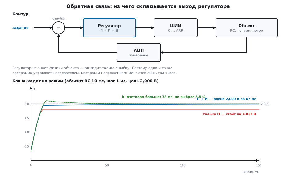
All the controller sees is the error: the difference between the setpoint and the measurement. It does not know what it controls: a heater, a motor or a voltage. That is why the same program works everywhere — only three coefficients and the period change.
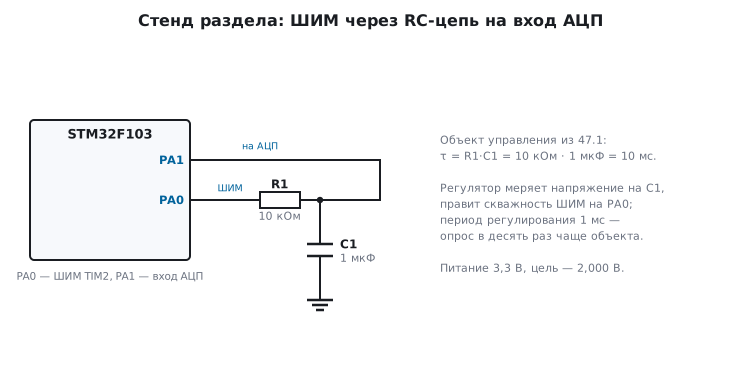
The analysis uses a model with easy numbers: PWM through an RC network with a time constant of 10 ms, a control period of 1 ms, a 3.3 V supply, a target of 2.000 V. In one period the output covers 9.5 % of the way to a new level.
47.2 P: the proportional part and its irremovable error
The simplest thing: the larger the error, the larger the output.
u = kP · (задание − измерение)
And right away the main property: with this kind of plant the error does not go to zero. This RC network, like a heater or a motor under load, needs a non-zero output to hold its level. If the error went to zero, the output would become zero and the plant would start to drop. Equilibrium is reached where the remaining error is exactly enough to hold the level:
| kP | Settled at | Shortfall |
|---|---|---|
| 1 | 1.535 V | 465 mV |
| 3 | 1.817 V | 183 mV |
| 5 | 1.886 V | 114 mV |
The model agrees with the formula v = kP·Vcc·target / (1 + kP·Vcc): the larger
kP, the smaller the remainder, but it never reaches zero.
A plant that integrates by itself — a shaft position, the level in a tank without
leaks — behaves differently: to stay in place it needs a zero output,
and a P controller brings it to zero error without an integral part.
The remainder can also be removed with a constant offset, u = u0 + kP·e, where u0 is the
output that holds the target (here 2 / 3.3 ≈ 61 % PWM). But the offset is correct
for one operating point only: change the load or the target — and the remainder
is back. The integral part (47.3) finds it by itself.
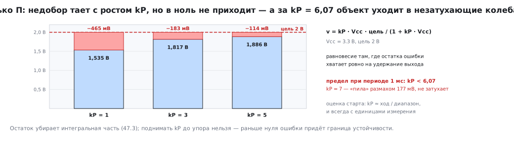
⚠️ The gain cannot be raised without limit. For this plant with a period of 1 ms, it stays stable while
kP < 6.07. At kP = 7 the output stops settling at all: undamped oscillations with a swing of 177 mV around the target. The sign on the oscilloscope is unmistakable — a steady "sawtooth" or sine wave that does not decay.
A starting estimate of kP. At the maximum error the controller is allowed
to output full travel: kP ≈ travel / range. With ARR = 1000 and a scale of
3.3 V this gives kP ≈ 300 if you work in volts, and 0.3 if in millivolts.
The coefficient is not a physical quantity: it links numbers, and its value
depends on the units of the input and output. Whenever you write down kP,
write down the units too.
47.3 I: the integral part removes the remainder
The error is accumulated. While it exists, the accumulator grows, and the output grows with it — until the error becomes zero.
накопитель += kI · ошибка · dt
u = kP · ошибка + накопитель
With kP = 3 and kI = 50 the model settles exactly at 2.000 V in 67 ms without overshoot. Quadruple kI — and it gets there in 38 ms, but with an overshoot of 5.8 %. This is the basic trade-off: faster means overshoot, smooth means slower.
The incremental form is also an integrator. The form
u += kP · errorwith kP = 0.05 is often called proportional control, but it accumulates, and therefore integrates: in the model it reaches exactly 2.000 V. The same kP = 0.05 in the positional formu = kP · errorgives only 0.283 V. The forms are not interchangeable, and their coefficients mean different things: in the incremental form kP plays the role of kI·dt.
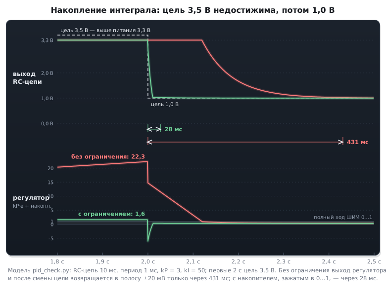
Windup with an unreachable target. If the target is beyond what is possible (3.5 V requested with a 3.3 V supply), the error does not go away, and the accumulator grows without bound. In the model the controller output grows to 22.3 (the accumulator itself to 21.7) — twenty-two times the full travel. When the target becomes reachable again, the controller keeps "working off" what it has accumulated for a long time:
| Return to normal operation | |
|---|---|
| accumulator not limited | 431 ms |
| accumulator limited | 28 ms |
A fifteen-fold difference. That is why you limit not only the output but also the accumulator itself, separately — the typical cause of "the controller is stuck at maximum" in finished devices.
47.4 D: the derivative part and why it is usually absent
The derivative reacts not to the size of the error but to how fast it changes: it helps catch the moment a load appears, before the error has grown.
The price is noise. The derivative amplifies it many times over:
| Swing in steady state | |
|---|---|
| P + I | 19.5 mV |
| P + I + D | 164.9 mV |
| P + I + D with filter | 17.6 mV |
| P + I with the same filter | 11.2 mV |
With measurement noise of ±10 mV (an ordinary ADC without averaging), adding the derivative makes the result eight times worse. A filter on the measurement brings it back to 17.6 mV, but it sits on the whole measurement and smooths the noise for P and I too: P + I with the same filter give 11.2 mV. So on a noisy signal the derivative part here does harm even with a filter. The filter also adds lag: after adding it, check the kP limit again. If the filter is needed only against derivative noise, put it on the derivative term alone.
The filter is a first-order lag, one line:
фильтр += k · (измерение − фильтр)
The coefficient is the ratio of the period to the desired time constant:
k = Ts / Tf. At 1 ms and 20 ms that is 0.05; the filter covers 63 % of a step in
20 ticks. k = 1 means no filter at all.
Take the derivative of the measurement, not of the error. Otherwise a setpoint step gives a kick: going from 0 to 2.000 V, the derivative of the error outputs 100 units of output instantly — saturation and a jerk of the actuator. The derivative of the measurement does not react to a setpoint change at all: the measurement did not jump.
In practice most tasks stop at a PI controller. The derivative part is added when the plant is inertial and slow (heating, large mechanics) and the measurement is clean.
47.5 A load step: what it is all for
The test the controller is built for. At tick 2000 the load takes a quarter of the output:
| Dip | Outcome | |
|---|---|---|
| P only | 237 mV | stayed at 1.763 V |
| P + I | 58 mV | returned to 2.000 V in 74 ms |
A proportional controller softens the blow but does not remove it. The integral part brings the quantity back to where it should be — that is its only job, but an irreplaceable one.
47.6 🔧 The controller in code
The three things people trip over most often: a constant period, limiting the accumulator, and the derivative of the measurement. All of it fits in twenty lines.
typedef struct {
    int32_t kp, ki, kd;          /* Q16 */
    int32_t integ;               /* Q16, накопитель */
    int32_t integ_max;           /* Q16, свой предел — не общий с выходом */
    int32_t prev_meas;           /* коды АЦП: производная берётся по измерению */
    int32_t filt;                /* Q16, фильтр измерения */
    int32_t k_filt;              /* Q16, коэффициент фильтра */
    int32_t out_min, out_max;    /* пределы выхода в шагах ШИМ */
} pid_t;

/* Один шаг. Вызывается строго с постоянным периодом — dt «зашит»
   в коэффициенты, и переменный период молча испортит настройку. */
int32_t pid_step(pid_t *p, int32_t target, int32_t meas)
{
    int32_t err, deriv, out;

    /* Фильтр измерения: без него дифференциальная часть работает по шуму. */
    p->filt += MUL_Q(p->k_filt, (meas << Q) - p->filt);
    meas = p->filt >> Q;

    err = target - meas;

    /* Интеграл со своим ограничителем: иначе при недостижимой цели
       он растёт без предела и потом долго «рассасывается». */
    p->integ = clamp(p->integ + p->ki * err, -p->integ_max, p->integ_max);

    /* Производная по измерению, а не по ошибке: смена задания не даёт броска. */
    deriv = -(p->kd * (meas - p->prev_meas));
    p->prev_meas = meas;

    out = ((p->kp * err) + p->integ + deriv) >> Q;
    return clamp(out, p->out_min, p->out_max);
}
Where to call it. In the interrupt handler of the same timer that generates the PWM, or on completion of an ADC conversion triggered by that timer (section 14.5). Not in the main loop: there the period "drifts", while all the coefficients are computed for a fixed one.
Bumpless transfer. If the controller is switched on while the plant is already running, preloading the accumulator with the current output is not enough. The filter and the previous measurement are at zero: the first step will filter the measurement starting from zero (with k = 0.05 you get 5 % of the real value) and take the derivative −kD · (measurement − 0) — exactly the kick that 47.4 warns about. And with a non-zero error, kP · error is added to the output as well. So you preload three things:
void pid_preload(pid_t *p, int32_t current_out, int32_t target, int32_t meas)
{
    p->filt      = meas << Q;               /* фильтр — с текущего измерения, а не с нуля */
    p->prev_meas = meas;                    /* первая производная — ноль */
    p->integ     = (current_out << Q) - p->kp * (target - meas);   /* П-часть + накопитель = current_out */
    p->integ     = clamp(p->integ, -p->integ_max, p->integ_max);
}
The first step after such a transfer starts exactly at current_out and adds
to it only the normal integral step kI · error.
47.7 Integers versus floating point
Quantities are kept in ADC codes, coefficients in Q16 format: an ordinary integer whose lower 16 bits are treated as the fractional part. Multiplication is a multiplication followed by a shift right by 16; division by a power of two is a shift.
#define Q            16
#define TO_Q(x)      ((int32_t)((x) * (1 << Q)))
#define MUL_Q(a, b)  ((int32_t)(((int64_t)(a) * (b)) >> Q))
The bit width is calculated, not guessed: kP = 3 in Q16 is 196608,
and its product with the full ADC scale (4095) still fits in signed
32 bits, while in Q20 format the same product already overflows.
A separate trap: integer division discards the remainder. The target
2.000 V in codes: 2000 × 4095 / 3300 gives 2481 instead of 2482 — the target is
0.8 of a code (about 0.66 mV) too low, and the controller will faithfully work off that error. The cure is
to add half the divisor: (a + b/2) / b.
Is it worth the trouble if you can write float? Measured by building the same
controller:
| Core | Integers | Floating point |
|---|---|---|
| Cortex-M3 (F103, no FPU) | 584 bytes | 1868 bytes |
| Cortex-M4F (F407, G474) | 616 bytes | 600 bytes |
On a core with a floating-point unit there is almost no difference — write float. On a core
without one, floating-point arithmetic pulls in a library and triples the
code, and loses even more noticeably in time. And do not use double
even on the M4F: the hardware unit there is single precision, and double is computed
in software.
47.8 How to tune
A method that works without theory:
- Set kI and kD to zero. Raise kP until the output starts oscillating without decay. Remember that value — call it the critical one.
- Take kP at about half the critical value. See what steady-state error remains.
- Add kI, starting from a small value, until the error goes away in an acceptable time. If overshoot appears, reduce kI or kP.
- kD — only if needed, and only together with a measurement filter. Raise it until the output first starts to "jitter", then halve it.
- Check the extreme cases: load applied and removed, a setpoint step, an unreachable target, switching the controller on while running.
While doing this, watch not the controlled quantity but the three terms separately — it is convenient to output them over SWO (section 21) or to the debugger: you immediately see which part oscillates and which has hit the limiter.
About the period. It must be noticeably shorter than the time constant of the plant — about ten times. Here it is 1 ms against 10 ms. Polling a heater with a time constant of minutes a thousand times a second is pointless: you only get noise and extra work.
47.9 Pitfalls
The quantity does not reach the setpoint. Only the proportional part, and the plant needs a non-zero output to hold its level. Steady-state error is its property, not a fault; you need the integral part.
Undamped oscillations. kP is above the stability limit of the plant, or the control period is too long.
The controller is "stuck" at maximum. The integral wound up while the target was unreachable. Limit the accumulator separately from the output.
Overshoot at start-up. The accumulator starts from zero and builds up while the plant catches up. Limit the accumulator, reduce kI, or on switch-on preload the accumulator, the filter and the previous measurement (47.6).
A jerk when the controller is switched on while running. Only the accumulator was preloaded, while the filter and the previous measurement stayed at zero: the first step takes the derivative from zero to the current measurement.
A jerk on a setpoint change. The derivative is taken of the error. Take it of the measurement.
The output jitters. A derivative part without a filter, or ADC noise. Filter the measurement, average the samples, check the ground and the reference (section 14).
The coefficients are "wrong" although the formula is right. The units were forgotten:
volts versus millivolts, codes versus percent, dt inside kI or
outside. Write the units next to the coefficient.
Works on the bench, fails in the product. The control period drifts: it is called from the main loop instead of an interrupt, or the handler is delayed by a longer interrupt (section 7.3).
Overflow in integer arithmetic. The product of a coefficient and the full scale does not fit. Calculate the worst case, and make the intermediate product 64-bit.
A half-step error out of nowhere. Integer division without rounding.
47.10 Summary
- The controller sees only the error — that is why one program can control anything; the specifics of the plant are hidden in three coefficients and the period.
- The proportional part leaves a steady-state error if the plant needs a non-zero output to hold its level (heating, an RC network); you cannot raise kP until the error is zero — stability is lost first.
- The integral part removes the error and brings the quantity back after a load step; the price of speed is overshoot.
- The accumulator is limited separately from the output — otherwise the return to operation takes an order of magnitude longer.
- A derivative part without a filter amplifies noise many times over; the derivative is taken of the measurement, not of the error; PI is enough for most tasks.
- Call it strictly with a constant period, roughly ten times shorter than the time constant of the plant.
- On a core without an FPU an integer controller is three times more compact than a floating-point one; on the M4F there is almost no difference.
- Tune step by step from kP to kI, checking the extreme cases and watching each term separately.
Next: section 48 "A custom bootloader and firmware updates" — how to change the program in a device that has already gone to the customer.