 Embedded HandbookApps
36л. Analyzers: logic, spectrum, network (NanoVNA) and bus
An oscilloscope shows voltage against time — and a little about almost everything. An analyzer answers one question, but answers it better. A logic analyzer tells you what is said on a bus: many channels, long records, only 0 and 1. A spectrum analyzer tells you which frequencies are in a signal and how strong they are, down to a weak line next to a strong one. A network analyzer tells you how an antenna, a filter or a cable reflects and passes a signal at each frequency. A bus analyzer tells you what went over CAN or USB, including errors that the software never sees.
The basics of the logic analyzer and PulseView are in 36а.6: the threshold, the rule of "four or five samples per bit", the protocol decoders. This section starts where they end. Oscilloscope triggering is in 36д, its FFT in 36е, bus decoding on the oscilloscope in 36ж.
The author has no documents for any specific analyzer. So the instruments are described by class: no model names and no numbers taken from other people's descriptions. There are two exceptions: the author's oscilloscope, RIGOL DHO900 (its documents are available), and a few general words about cheap FX2-based dongles under sigrok. Every calculated number comes from a model.
Sources: RIGOL DHO900 Datasheet (Books/dho900-datasheet.pdf; page numbers
are PDF file pages): p. 4 and 9 — 16 digital channels and the PLA2216 logic probe,
p. 11–12 — digital channels, p. 17 — FFT, p. 18–19 — decoding and the
Bode plot, p. 26 — notes 6 and 7; DHO900 User Guide
(Books/DHO900_UserGuide_EN.pdf): p. 69 and 74 — restrictions, p. 138 —
FFT units, p. 177–179 — the digital channel menu. All calculated numbers are a
run of _verify/anl36l/model36l.py (Python 3.11 and numpy in the
stm-lab:1 container).
What it is called in the documentation
Original Meaning sample rate; timing / state analysis how often inputs are sampled; sampling on the analyzer's own clock or on an external clock memory depth, streaming, RLE samples held in the instrument, continuous transfer to the PC, run-length encoding threshold, hysteresis level that separates low from high; separate rising and falling levels protocol decoder, stacked decoder turns levels into protocol data; a decoder that works on top of another pattern trigger, sequential trigger trigger on a combination of channels; trigger on A followed by B swept / FFT spectrum analyzer analyzer that tunes a filter across the span; analyzer that digitizes a band at once RBW, VBW, span, sweep time resolution bandwidth, video filter, frequency range shown, time to cover it noise floor, DANL; detector the analyzer's own displayed noise; how each display point is formed input attenuator, reference level attenuation before the mixer; level at the top of the screen near-field probe, pre-compliance small loop or stub that finds emission sources; EMC screening before the lab SDR, I/Q software-defined radio; quadrature samples VNA; S11, S21 vector network analyzer; reflection and transmission reflection coefficient, VSWR, return loss, mismatch loss Γ, standing wave ratio, reflection in dB, power lost to reflection Smith chart chart of the reflection coefficient plane SOLT calibration, reference plane short, open, load, through calibration; point where the measurement starts L-match two-element matching network bus / protocol analyzer, sniffer instrument or node that records bus traffic
36л.1 Logic analyzer: what happens between samples
What it is. A logic analyzer compares every input with a threshold at equal intervals and stores 0 or 1. Between samples it is blind — so any moment in the record is known only to within one sample period, and a pulse shorter than that period can disappear.
Model. The class of cheap dongles from 36а.6 — 24 MS/s, a step of 41.7 ns. The signal arrives at a random phase with respect to the samples:
| at the input | in the record |
|---|---|
| a 20 ns pulse | seen in 48.1 % of records (calculation 48.0 % — width divided by the step) |
| a 50 ns pulse | always seen; its length in the record is 41.7 ns (80.2 % of records) or 83.3 ns (19.8 %) |
| two edges 10 ns apart | simultaneous in 76.0 % of records, 41.7 ns apart in 24.0 % |
| SCK 8 MHz: 3 samples per period | the 62.5 ns high level is shown by one sample in 50.2 % of periods and by two in the rest — duty cycle 33 or 67 % instead of 50 |
What follows. The width of a pulse in the record is always a whole number of steps. Only a pulse no shorter than one step is seen reliably. Times are measured with an error of up to one step either way. At 24 MS/s an SPI clock is fine up to 6 MHz (four samples per period); above that you need a faster analyzer or an oscilloscope.
State mode. Some analyzers can take a sample not on their own clock but on an edge of an external clock signal — for example, on SCK. The record then holds the bus value at each clock, and no time at all. Whether a given instrument has this mode is in its documentation.
Mistake. Measuring pulses comparable with the step and trusting the third digit. A 50 ns width is recorded as 41.7 or 83.3 ns — it will not get more accurate than that.
36л.2 Memory and streaming over USB
Two designs. Some analyzers have their own memory: the record goes there at full rate and is then uploaded. Its length is limited by the depth: 1 million samples at 24 MS/s is 41.7 ms. Others have almost no memory: every sample goes straight to the PC as a stream. The record length is then limited only by the disk, but the sample rate is limited by the bus.
Streaming. 8 channels at 24 MS/s is 24 MB/s; 16 channels is 48 MB/s. USB 2.0 is nominally 480 Mbit/s, that is 60 MB/s, but bulk transfers by the specification fit at most 13 packets of 512 bytes into a 125 µs microframe — 53.248 MB/s. 16 channels at 24 MS/s would take 90.1 % of that ceiling — on a real PC, with other devices on the bus, this is out of reach. One hour of recording at 24 MB/s is 86.4 GB.
FX2 dongles. Cheap clones built on the CY7C68013A (FX2) chip under sigrok work exactly this way: it is a USB 2.0 controller with a small buffer, there is no memory for the record, and the sample rate is limited by USB 2.0 and by whether the PC keeps up with the stream. If it does not, the record stops or loses pieces — how exactly depends on the software.
Compression. Slow signals hardly change, so instead of samples you can store the lengths of runs of equal values (RLE). Model: 1 s of UART at 115200 baud, the line continuously busy with random bytes, 24 MS/s — 24.00 million samples (24 MB) give 63706 runs; at 5 bytes per run (a state byte and 4 length bytes) that is 319 KB — 75 times less. A fast, busy bus compresses badly, a slow one compresses very well. Whether a given instrument compresses, and at which stage, is in its documentation.
Mistake. Setting the highest sample rate for an hour-long record of a slow UART: the stream hits the bus limit and the disk fills up, while 115200 baud would be fine at 1 MS/s (8.7 samples per bit, 36а.6).
36л.3 Threshold, levels and loading of the line
Threshold. How to choose it for 3.3 and 1.8 V is in 36а.6; the DHO900 threshold presets and the "threshold does not match the logic" mistake are in 36д.6. Cheap dongles usually have one fixed threshold of the input chip; better instruments have comparators with a settable threshold. Hysteresis (the rising threshold above the falling one) is needed for slow edges — 36л.6.
Input limit. Every instrument has its own, and it is written in its documents. Example — the DHO900 digital inputs: up to ±40 V peak, CAT I; the signal swing at least 500 mV peak-to-peak (datasheet p. 11). Dongles without an input buffer can have a lower limit — without a document, apply neither a negative voltage nor anything above the logic supply to the input.
Loading. An analyzer input is a resistance and a capacitance on the line. The DHO900 logic probe has about 101 kΩ and about 8 pF (datasheet p. 11). The current through 101 kΩ from 3.3 V is 32.7 µA; a push-pull output does not care. But 8 pF on an I²C line with a 4.7 kΩ pull-up is a time constant of 37.6 ns, that is, its own 10 to 90 % edge of 82.6 ns, and it adds to the bus capacitance (160.5). At 100 kHz this is negligible; in fast I²C modes it is noticeable. High-impedance nodes (a crystal, an RC network) are not touched with an analyzer probe at all.
Ground. Long flying leads without a ground nearby ring in the same way as the ground lead of an oscilloscope probe (36а.2): the ringing crosses the threshold, and extra edges appear in the record. Ground for every group of channels, short leads.
36л.4 Decoders and how they stack
What it is. A protocol decoder turns levels into meaning (36а.6). In sigrok and PulseView decoders stack: the lowest one turns levels into bytes (I²C, SPI, UART), the next one on top turns bytes into operations of a specific chip: an EEPROM, a sensor, an SPI flash memory. USB has several such layers: from line levels to packets and from packets to requests. The sigrok decoders are written in Python, and your own layer on top of an existing one is written following the neighbouring ones.
Model. Two layers on one record: I²C at 100 kHz sampled at 1 MS/s (10 samples per bit), an EEPROM at address 0x50 with a two-byte cell address. First two bytes are written, then read back. The lower layer gives I²C events, the upper one (after "--") what was done to the memory:
START
  A0 ACK
  00 ACK
  10 ACK
  41 ACK
  42 ACK
STOP
START
  A0 ACK
  00 ACK
  10 ACK
START
  A1 ACK
  41 ACK
  42 NACK
STOP
--
запись по 0x0010: 41 42
чтение с 0x0010: 41 42
The second layer understands what the first one does not: a repeated START with the read bit after two address bytes is a read from address 0x0010, and NACK on the last byte means the master ended the read itself, not an error.
Mistake — decoder settings. 0xA0 and 0x50 are the same address: the first with the R/W bit, the second without (the DHO900 can also show the address either way, datasheet p. 18). UART without the right baud rate, data bits, parity and polarity, SPI without the right CPOL, CPHA, bit order and CS polarity give plausible garbage. If the decode is "almost right", check the settings, not the board.
36л.5 Triggering
What it is. The condition that starts the record: level 0 or 1, a rising, falling or any edge — on any channel and on a combination of channels (a pattern). Better instruments have a sequential trigger (first A, then B) and a trigger on a value in the decoded protocol (an I²C address, a CAN identifier). On dongles without their own memory the condition is checked by the software on the PC, on the stream; on instruments with memory — by the instrument itself. The pre-trigger record is a share of the memory set in advance.
Model. The same I²C record, 1.16 ms. A "falling edge on SDA" trigger fires 21 times — on every bit transition from 1 to 0. The START condition (SDA falls while SCL = 1) fires 3 times: two STARTs and one repeated START. You need a two-channel pattern, not an edge on one channel.
Mistake. Triggering on a single edge on a bus: the instrument fires on the first bit that comes along, and the frame you want ends up outside the record. The DHO900 has a bus trigger for this (36д.19).
36л.6 What a logic analyzer does not see: a runt and a slow edge
Runt. A pulse that did not reach the full level (36д.14). Model: a 0 → 1.2 V → 0 triangle 40 ns long, 24 MS/s. With a 1.5 V threshold it never exists. With a 1.0 V threshold it stays above the threshold for 6.67 ns — it appears in 16.1 % of records (calculation 16.0 %) and looks there like an ordinary 41.7 ns pulse, indistinguishable from a full one. The question "did the level make it" is not asked of a logic analyzer — it only answers "0 or 1".
Slow edge. A 10 µs edge from 0 to 3.3 V with 30 mV of noise on it, threshold 1.5 V:
| record | extra transitions on the edge | mean transitions | largest |
|---|---|---|---|
| 24 MS/s, 240 samples per edge | in 62.7 % of edges | 2.6 | 7 |
| 625 MS/s | in 100.0 % of edges | 63.7 | — |
| 24 MS/s, hysteresis ±0.1 V | never | 1 | 1 |
The noise carries the signal across the threshold back and forth several times, and the decoder sees extra bits. A fast analyzer is worse here than a slow one: it catches every crossing. Hysteresis (or a Schmitt trigger on the line) fixes it, not the sample rate.
The threshold shifts time. On the same 10 µs edge a 1.4 V threshold and a 1.65 V threshold give moments 757.6 ns apart. Two instruments with different thresholds disagree by the same amount when measuring a delay.
What to do. Analog questions — level, shape, whether it got there — go to the oscilloscope: a runt is caught by the Runt trigger (36д.14), a slow edge by the rise time measurement (36е.10). Best of all, both kinds of channels on one time axis (36л.19).
36л.7 Spectrum analyzer: resolution bandwidth and noise floor
What it is. An instrument that measures power at each frequency. A classic swept analyzer shifts the input with a mixer to an intermediate frequency and passes it through a narrow filter — the resolution bandwidth (RBW); by tuning the local oscillator it moves this filter across the whole frequency span. The main settings: center and span (or start and stop), RBW, video filter VBW, reference level, attenuator, sweep time.
RBW separates close frequencies. Model — a filter with a Gaussian response, two equal tones 10 kHz apart:
| RBW | dip between the tones |
|---|---|
| 3 kHz | 30.4 dB — two separate peaks |
| 10 kHz | 0.33 dB — barely visible |
| 20 kHz | 0.00 dB — one hump |
RBW sets the noise floor. Noise enters the filter in proportion to its width. Model (white noise through the same filter): from 1 to 10 kHz the floor rises by 9.99 dB, from 10 to 100 kHz by 10.00 dB; the calculation is 10·lg 10 = 10.00 dB for every tenfold step. The lower limit is thermal noise: at 290 K it is −173.98 dBm per hertz, in a 10 kHz bandwidth −133.98 dBm; the analyzer's own noise adds to it, and that has to be taken from the documents of the specific instrument. You see a weak signal by narrowing the RBW.
The price is time. A narrow filter responds slowly, and it has to be moved across frequency slowly: sweep time ≈ k·(span)/RBW². Model — a tone passing through a Gaussian filter at different speeds:
| k | amplitude error |
|---|---|
| 0.5 | −1.25 dB |
| 1 | −0.39 dB |
| 2.5 | −0.07 dB |
| 10 | 0.00 dB |
With k = 2.5 a 100 MHz span is covered with a 100 kHz RBW in 25 ms, with a 10 kHz RBW in 2.5 s, with a 1 kHz RBW in 250 s. That is why analyzers usually couple the sweep time to the RBW by themselves.
Mistake. Shortening the sweep time by hand at a narrow RBW: the peaks come out lower than they are and drift in frequency. If the instrument warns about an uncalibrated mode, this is it.
36л.8 Detector and video filter (VBW)
What it is. After the RBW filter come a detector (peak, sample, average) and a logarithmic scale, and after them the VBW video filter, which smooths the trace on the screen.
Model — noise on a logarithmic scale. The envelope of noise after a narrow filter has a Rayleigh distribution. Its logarithm, averaged, lies 2.51 dB below the true noise power. Without smoothing the noise trace jitters with a standard deviation of 5.57 dB; smoothed over 100 independent points it is 0.56 dB.
Why VBW. The video filter makes the trace thinner and reveals a weak steady line in the noise, but it does not lower the floor itself — RBW does that (36л.7). Mistake: measuring the noise level with the peak detector (it shows the spikes) or by the averaged logarithm (it reads low by 2.51 dB). For noise, use a power-averaging detector, if there is one.
36л.9 Swept or FFT; the attenuator and the analyzer's own harmonics
A swept analyzer looks at one frequency at a time. Span 100 MHz, RBW 100 kHz, sweep 25 ms: the filter stays on each frequency for 25 µs. A 1 ms burst from a radio sensor every 100 ms falls into a sweep with a probability of 1.025 %: on average one catch per 97.6 sweeps, about 2.44 s — if the sweep and the bursts are unrelated. If the sweep period is a multiple of the burst period, the instrument may never see it at all. Max hold and patience help.
An FFT analyzer (and an SDR, 36л.12) digitizes a whole band at once and sees every burst inside it. A wide span is also covered in steps — there is no miracle beyond its instantaneous bandwidth.
Its own harmonics. The mixer is nonlinear: on a strong signal the instrument creates harmonics itself. The second harmonic created inside grows by 2 dB for every decibel of input, that is, relative to the fundamental (in dBc) by 1 dB per decibel. Model: the signal has a second harmonic at −70 dBc, and with the attenuator at 0 dB the analyzer adds its own at −50.00 dBc:
| attenuator | second harmonic on the screen |
|---|---|
| 0 dB | −49.96 dBc |
| +10 dB | −59.59 dBc |
| +20 dB | −66.99 dBc |
| +30 dB | −69.59 dBc |
The test. Add 10 dB of attenuation. If the harmonic in dBc has not changed, it is in the signal; if it dropped, the instrument draws it. The price: every 10 dB of attenuation raises the noise floor by the same 10 dB.
Input limit. The maximum power and DC voltage at the input are given in the instrument's documents. The DC component is blocked with a series capacitor (a DC block), a powerful output with an external attenuator. A transmitter output is never connected straight to the analyzer input.
36л.10 Spectrum analyzer versus oscilloscope FFT
The oscilloscope FFT (36е.21–36е.23) and a spectrum analyzer draw a similar picture, but they work differently:
| oscilloscope FFT | spectrum analyzer | |
|---|---|---|
| input | 1 MΩ (the only one on the DHO900, 36г.6); 50 Ω with a feedthrough terminator | 50 Ω, levels in dBm |
| what the ADC sees | the whole band at once: a strong signal sets the scale, a weak one lives in the remaining bits | a narrow band after the mixer and filter |
| top frequency | half the sample rate and the channel bandwidth | its own range, independent of the time base |
| resolution | inverse of the record length; the DHO900 FFT takes no more than 1 million points (datasheet p. 17) | RBW |
| link to time | the same record: a line can be tied to an event | none |
Model — what 12 bits give. An ideal 12-bit ADC with a full-screen sine: the quantization signal-to-noise ratio is 74.0 dB. This noise is shared among the FFT bins: with 65536 points and a Hanning window it is −116.6 dBc per bin (calculation −117.4), with 1 million points −129.2 dBc. In theory the floor is very low; in practice it is set by the instrument's own noise and spurious lines, which the DHO900 documents do not give (36г.3).
Units. The DHO900 offers dBm, dBV or Vrms (User Guide p. 138; 36е.22). 0 dBm into 50 Ω is 223.6 mV RMS, or 107.0 dBµV: EMC limits are written in dBµV.
When to use which. Low frequencies, tying a line to an event in time, ripple and pickup — the oscilloscope FFT. Weak next to strong, radio bands, transmitter harmonics, EMC — the spectrum analyzer.
36л.11 EMC before the lab: the near-field probe
Who emits in a device is in 203.2, the check with a receiver next to the board in 203.6, the order "own bench, then lab" in 206.5. A spectrum analyzer (or an SDR) with a near-field probe adds the main thing: where the source is — which trace, which chip, which cable.
What it is. A magnetic probe is a small loop at the end of a coaxial cable. The voltage on it is proportional to frequency and to the magnetic flux through the loop. Model: a 10 mm square loop 2 mm from a trace carrying 10 mA:
| frequency | voltage on the loop |
|---|---|
| 10 MHz | 2.25 mV, 67.0 dBµV |
| 100 MHz | 22.52 mV, 87.0 dBµV |
The response rises by 20 dB per decade. Hence a trap: in an 8 MHz square wave the harmonic current falls as 1/n (the ninth is at −19.1 dB to the first), while the probe boosts it n times — and all odd harmonics appear at the same level, 0.0 dB to the first. The spectrum through a probe is not the field at three metres from the standards, but a map of the sources on the board.
How to use it. Only "before and after" comparison: the same spot, the same height above the board, the same RBW and attenuator. Once the source is found, slow the edge, add a ferrite bead, move the trace next to ground — and see by how many decibels the line dropped. An electric probe (a short stub) finds radiating cables and high-voltage nodes. An absolute level against the limits comes only from a test site with a calibrated antenna (203.7, 206.5).
Mistake. Comparing readings taken at different probe heights: in the near field the level depends strongly on distance, and an "improvement by 10 dB" turns out to be a moved hand.
36л.12 SDR and low-cost analyzers as a class
SDR. A receiver with a tunable local oscillator and an ADC that sends the PC a stream of quadrature samples (I/Q); the software computes the spectrum. The instantaneous bandwidth is of the order of the sample rate; a wide span is assembled by the software, retuning piece by piece.
What the class has in common. A frequent 8-bit ADC: the ideal quantization signal-to-noise ratio is 49.9 dB against 74.0 dB for 12 bits. A strong signal nearby overloads the chain, and lines that are not there appear. In the center of the band there is often a line from local oscillator leakage and DC offset, at the edges mirror images. There is usually no absolute level calibration: the dBm on the screen are nominal.
What it is good for. "Before and after" comparison (203.6, 206.5), finding a carrier and its harmonics, watching the air at the frequency of your own radio, work with a near-field probe. Low-cost swept analyzers and FFT analyzers come with the same class of caveats; their specifications come only from their documents.
Mistake. Taking a line exactly in the center of the SDR band for a signal. Shift the tuning frequency: a real line stays at its frequency, a false one moves with the center.
36л.13 Network analyzer: S11, S21 and the Smith chart
What it is. A vector network analyzer (VNA) sweeps a sine wave in frequency itself and at each frequency measures the amplitude and phase of the waves: reflected from the circuit input (S11) and passed through it (S21). A scalar instrument measures amplitude only. NanoVNA is a class of small two-port analyzers with an open design, a screen and USB: the first port transmits and measures reflection, the second receives what passed — S11 and S21; the reverse direction is measured by turning the circuit around. Ranges and accuracy differ between units of this class; they are not given here — only from the documents of the specific instrument.
The Smith chart. The plane of the reflection coefficient Γ: the center is exactly 50 Ω, the left edge is a short circuit, the right edge an open circuit; the upper half holds inductive impedances, the lower half capacitive ones. Circles around the center are constant VSWR. A circuit swept in frequency draws a curve on it: a series resonant circuit crosses the horizontal axis at its resonant frequency (figure in 36л.16).
Mistake. Looking only at the VSWR curve: it loses the sign of the reactance, and you cannot see whether an inductor or a capacitor is needed for matching. The Smith chart shows it.
36л.14 Reflection coefficient, VSWR and return loss
Formulas. Γ = (Z − 50)/(Z + 50); VSWR = (1 + |Γ|)/(1 − |Γ|); return loss = −20·lg|Γ|; mismatch loss = −10·lg(1 − |Γ|²); reflected share of power — |Γ|².
| load | Γ | VSWR | return loss | reflected | mismatch loss |
|---|---|---|---|---|---|
| 75 Ω | 0.200 | 1.50 | 13.98 dB | 4.0 % | 0.18 dB |
| 100 Ω | 0.333 | 2.00 | 9.54 dB | 11.1 % | 0.51 dB |
| 25 Ω | −0.333 | 2.00 | 9.54 dB | 11.1 % | 0.51 dB |
| 150 Ω | 0.500 | 3.00 | 6.02 dB | 25.0 % | 1.25 dB |
The mismatch loss at VSWR 2 and 3 is the same 0.51 and 1.25 dB as in 92.5. 25 and 100 Ω give the same VSWR: it does not tell you which way the error goes — the complex Γ does.
Mistake — signs. Return loss is a positive number (9.54 dB), S11 in decibels is the same with a minus sign (−9.54 dB). "Return loss −10 dB" and "S11 = −10 dB" mean the same thing, but a phrase like "a loss of 10 dB is worse than 20 dB" is true only for return loss: the larger, the better the match.
36л.15 SOL(T) calibration
Why. Without calibration the analyzer measures not only the circuit but also its own bridge, connectors and cable. The reflection errors are described by three complex numbers: directivity e00, port match e11 and reflection tracking e01: Γmeas = e00 + e01·Γ/(1 − e11·Γ). Three unknowns — three known loads: a short circuit (Γ = −1), an open circuit (+1), a 50 Ω load (0) — SOL calibration. For S21 a jumper between the ports is added (Through, T) — transmission normalization.
Model. Nominal bridge and cable errors:
| load | VSWR without calibration | after SOL |
|---|---|---|
| exactly 50 Ω | 1.17 | — |
| 75 Ω (true VSWR 1.50) | 1.26 | 1.500 |
| 150 Ω (true VSWR 3.00) | 2.36 | 3.000 |
Reference plane. You calibrate where the circuit connects: at the end of the cable, of the adapter, at the pads on the board. Model: after calibration 10 cm of cable were added (velocity factor — a nominal 0.66). At 868 MHz Γ rotates by 316°, and a 75 Ω load shows as 63.7 + j18.5 Ω. The VSWR stays 1.50: a lossless cable keeps the VSWR, but not the impedance.
Mistake. Calibrating over one range or with one number of points and measuring over another; calibrating without the cable and measuring through it; not repeating the calibration after warm-up and after changing an adapter. The calibration loads themselves are not ideal either — for cheap kits their corrections are unknown, and that is the limit of accuracy.
36л.16 Matching an antenna with an L-match
Antennas are a separate topic (92.5, 93); here — how a network analyzer helps to match one.
Antenna model. A series resonant circuit: 20 Ω, resonance at 920 MHz — an antenna for the wrong band. At the working 868 MHz its impedance is 20.0 − j40.4 Ω: |Γ| = 0.622, VSWR 4.30, return loss 4.12 dB, mismatch loss 2.13 dB. VSWR is below 2 nowhere: the best, 2.50, is at 920 MHz.
Length first. If the antenna can be shortened or lengthened, first move the resonance to the working frequency, and only then match what is left.
L-match. The antenna resistance is below 50 Ω — so one element goes in series with the antenna and one in parallel on the 50 Ω side. The network Q = √(50/20 − 1) = 1.225. In series you need a total of Q·20 = 24.49 Ω of reactance; the antenna has −40.4 Ω of its own, so add +64.88 Ω — an inductor of 11.90 nH. In parallel: −50/Q = −40.82 Ω — a capacitor of 4.49 pF. Check by calculation: the input is 50.00 + j0.00 Ω, VSWR 1.000. With the nearest E12 values — 12 nH and 4.7 pF — the VSWR is 1.07, return loss 29.2 dB. VSWR is below 2 from 852 to 884 MHz, a bandwidth of 32.0 MHz.
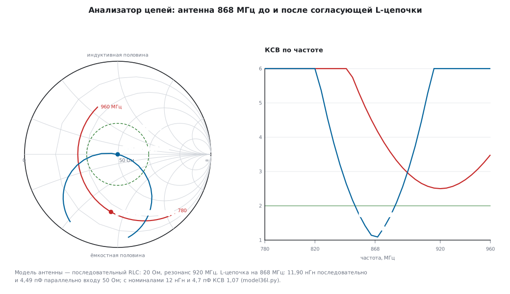
On the board. At 868 MHz the pads, vias and the parts themselves have their own parasitic inductance and capacitance, so the calculation is only a starting point: after soldering you measure with the analyzer and tune. Calibrate at the antenna connector or at the pads. Measure in the enclosure and in the hand — the enclosure and the hand shift the resonance; antenna placement is in 92.5. For matching three footprints are usually left (a pi network), so that either of the two L-matches can be fitted without changing the board.
Mistake. Matching the antenna on the bench without the enclosure: in the enclosure the resonance moves, and the tuned network becomes a mismatching one.
36л.17 Measuring a filter
How. S21 is how much passes, S11 how much is reflected at the input. Calibration — SOLT, together with the cables that connect the filter.
Model. A third-order Butterworth low-pass filter, 100 MHz, 50 Ω: 31.83 pF — 159.2 nH — 31.83 pF.
| frequency | S21 | return loss at the input |
|---|---|---|
| 50 MHz | −0.07 dB | 18.1 dB |
| 100 MHz | −3.01 dB | 3.0 dB |
| 200 MHz | −18.13 dB (calculation −18.13) | 0.1 dB |
| 300 MHz | −28.63 dB | 0.0 dB |
What you see. In the stopband a reactive filter does not absorb but reflects: the return loss is near zero — the power goes back to the source. The depth of the stopband is limited by the analyzer itself — its dynamic range and leakage between the ports: a flat shelf at the bottom of the S21 curve is the limit of the instrument, not of the filter.
Low frequencies. Audio filters and filters in front of an ADC (178) are easier to measure with the Bode plot on the oscilloscope: on the DHO914S and DHO924S from 10 Hz to 25 MHz (datasheet p. 19, 26; 36е.24), the generator is in 36к.
36л.18 Bus analyzers: CAN, USB and protocol analyzers
CAN. A CAN analyzer is a node with a CAN controller in "listen only" mode: timestamps, error frames, bus load, filters, often transmission too. A home-made version is the 198е sniffer (SLCAN, silent mode) and an adapter with SocketCAN — 19ж. A logic analyzer on the RX output of the transceiver also reads CAN: 500 kbit/s at 24 MS/s is 48 samples per bit, the bits and stuff bits are visible. But it has no controller error counters, and the record is limited.
Model — bus load. A frame with identifier 0x123 and 8 bytes 11…88: 111 bits without stuff bits (including the 3-bit interframe space), stuff bits — 1, total 112 bits; in the worst case of stuffing, 135 bits. 1000 such frames per second at 500 kbit/s is a load of 22.4 %. An analyzer shows it at once; it decides whether low-priority frames get through (19.3).
USB — three levels. - Software on the PC (USB capture in the operating system, decoding in Wireshark) sees requests the way the host stack sees them. It does not see electrical signals, retries and NAKs handled by the host controller, and nothing at all if the device did not pass enumeration. - A hardware protocol analyzer is inserted into the cable between host and device and records every packet with its time, including errors and NAKs. This is the tool for debugging your own USB device (20, 20д). - A logic analyzer. Low speed 1.5 Mbit/s at 24 MS/s is 16 samples per bit, readable. Full speed 12 Mbit/s — a bit is 83.3 ns, 2 samples per bit: below the rule of 36а.6, you need 48 MS/s or more. High speed 480 Mbit/s — a bit is 2.08 ns: beyond this class, only a dedicated analyzer.
Protocol adapters for I²C and SPI can not only listen but also drive the bus themselves: talk to a chip from the PC, even before there is firmware.
Mistake. Looking in the PC capture for the reason the device "is not detected": things never got as far as the driver, and the capture is empty. You need a hardware analyzer here, or at least an oscilloscope on D+ and D− (20.5).
36л.19 The DHO900 as an analyzer
What follows applies only to the DHO900, according to its documents.
16 digital channels. D0–D15 are present on every model, but the PLA2216 logic probe is bought separately (datasheet p. 4, 9). It must not be plugged in or pulled out while the instrument is on (User Guide p. 177). The threshold is set separately for D0–D7 and D8–D15 (User Guide p. 178) — from −15 to +15 V in 10 mV steps, with ready-made thresholds for logic families (datasheet p. 11; how to choose — 36д.6). The input is about 101 kΩ and about 8 pF (36л.3).
Speed. The shortest detectable pulse is 5 ns, the highest input frequency 200 MHz, the skew between digital channels ±5 ns (datasheet p. 12); the condition for it is a digital channel sample rate of 625 MSa/s, that is, a step of 1.6 ns (datasheet p. 26, note 6). This is 26 times faster than the 24 MS/s class of 36л.1. The memory depth of the digital channels is not given in the documents.
Before work. When the probe is connected for the first time and when the temperature changes by more than 5 °C, the probe is calibrated (ProbeCalibration, User Guide p. 179). Digital channels cannot be used together with averaging (User Guide p. 69) and are not available in Roll mode (User Guide p. 74).
The main advantage. Analog and digital channels share one time axis and one trigger. This is the answer to 36л.6: put the suspicious line on an analog channel with the Runt trigger (36д.14), the bus on digital channels. You can also trigger from D0–D15 (36д.6).
Decoding. Up to 4 protocols at once: Parallel, RS232/UART, I2C, SPI, LIN and CAN, source CH1–CH4 or D0–D15 (datasheet p. 18–19). Details are in 36ж.
As a spectrum analyzer — FFT in Math: up to 1 million points, six windows, a search for up to 15 peaks (datasheet p. 17), units dBm, dBV or Vrms (User Guide p. 138); how to use it is in 36е.21–36е.23. The input is 1 MΩ only (36г.6).
As a network analyzer at low frequencies — the Bode plot on the DHO914S and DHO924S (datasheet p. 19; note 7 on p. 26): 36е.24.
What it does not replace. A bus record many hours long (that is a stream to the PC, 36л.2), radio frequencies above the channel bandwidth — 125 or 250 MHz (datasheet p. 9), a network analyzer in the radio range.
36л.20 STM32 as a simple analyzer
- A logic analyzer from a BluePill — mini-project 198д: eight channels, up to 4.5 MS/s, a ring of 16384 samples, decoding and export for PulseView. It also explains why it cannot go faster.
- A CAN sniffer — 198е; an adapter for SocketCAN — 19ж.
- One frequency instead of a spectrum — the Goertzel algorithm (81б) on ADC samples: "is there a tone and how strong" without a full FFT; filters — 81а. A generator on an STM32 for measurements — 36к.
Such an instrument is for understanding how things work and getting the job done while you have no real one. The inputs have no protection, with the limits of the pin itself (198д.1).
36л.21 Pitfalls
The pulse is there one moment and gone the next. Shorter than the sample step: 20 ns at 24 MS/s is seen in 48.1 % of records (36л.1).
The square wave duty cycle "jumps". Three samples per period: SCK 8 MHz is shown as 33 or 67 % (36л.1).
Extra bits on a slow line. The noise carries the edge across the threshold back and forth: in 62.7 % of edges at 24 MS/s. Hysteresis or an oscilloscope (36л.6).
The runt is not visible. A logic analyzer answers "0 or 1" — a 1.2 V runt does not exist with a 1.5 V threshold (36л.6).
The record stops. The stream does not fit into USB 2.0: 16 channels at 24 MS/s is 90.1 % of the bulk transfer ceiling (36л.2).
The decode is plausible garbage. Wrong decoder settings: address with or without the R/W bit, CPOL and CPHA, UART baud rate (36л.4).
Peaks are lower than they should be. The sweep time was shortened by hand: at k = 0.5 the error is −1.25 dB (36л.7).
A harmonic "in the signal". The analyzer's mixer draws it: +10 dB of attenuation, and it dropped from −49.96 to −59.59 dBc (36л.9).
A line exactly in the center of the SDR. Local oscillator leakage, not a signal (36л.12).
VSWR 1.26 on a 75 Ω load. Not calibrated: it is really 1.50 (36л.15).
Matched on the bench, worse in the enclosure. The enclosure and the hand shift the resonance; measure the assembled device (36л.16).
The USB capture is empty. The device did not pass enumeration — the software on the PC does not see it (36л.18).
36л.22 Summary
- A logic analyzer knows time to within one sample step: a pulse shorter than the step disappears, a width in the record is a whole number of steps.
- Streaming over USB 2.0 is limited to 53.248 MB/s of bulk transfers — hence the sample rate of FX2 dongles; own memory gives speed but a short record. Slow signals compress well as run lengths.
- Decoders stack: levels → bytes → chip operations. Trigger on a pattern, not on a single edge.
- A runt and a slow edge are questions for the oscilloscope; extra transitions are cured by hysteresis, not by the sample rate.
- Spectrum analyzer: RBW separates close frequencies and lowers the floor by 10 dB per decade, but the sweep time grows as its square. VBW smooths, but does not lower the floor. Its own harmonics are given away by the attenuator test.
- A near-field probe shows where the source is and emphasizes high frequencies; it is good for "before and after", not for the limits.
- Network analyzer: Γ, VSWR and return loss are the same thing in different words; SOL(T) calibration at the connection plane is mandatory. An L-match of 11.90 nH and 4.49 pF matches the antenna model at 868 MHz.
- A bus analyzer sees what is not in the software: CAN errors, NAKs and USB enumeration.
- The DHO900 puts analog and 16 digital channels on one time axis; its FFT and Bode plot are in 36е.
Next: section 36м "Higher-end RIGOL oscilloscopes: DHO1000 and DHO4000 — what they add and how remote control differs" — how the senior models differ from the DHO900 and how to port a script to them.