 Embedded HandbookApps
121д. Industrial TinyML cases: motor, pump and fan condition, leaks by sound, counting and detecting objects in a frame — what was solved, with what, and where it went wrong
Sections 116–121г covered the tools one at a time: models, features, training, quantization, inference on the board, anomalies, sound, the camera and the whole path from a task to a device. This section takes five typical shop-floor tasks as cases: a motor, a pump, a fan, a compressed-air leak and counting parts on a conveyor. For each: the task and the cost of an error, the sensor and where to mount it, the sample rate and window, the features, the model, its cost on the F407, the acceptance measure and, above all, what broke when moving from the training data to the field and how it was fixed.
The data are synthetic but built from the physics of each task: bearing-defect impacts at the BPFO and BPFI frequencies, cavitation as bursty broadband noise, the blade pass frequency of a fan, the turbulent ultrasound of a leak, parts on a belt with changing light and glare. The seed is fixed, so every number repeats. These are not data from real plants: the cases show which errors happen and how to catch them, not what accuracy to expect on your motor.
Sources: numpy 2.3.3 and scikit-learn 1.7.2 in the stm-ml:1 image (as in
sections 116 and 118) — data, features, training; our own C inference
(infer121f.c) — features from the raw window and the model answer, checked
against Python with gcc 12.2.0 in the stm-sys:1 image; armclang from Keil MDK
5.43 — code and buffer sizes for the Cortex-M4F.
Terms used in the documentation
Term Meaning condition monitoring watching the state of a machine unbalance, misalignment mass off the shaft axis; shafts not in line BPFO, BPFI (ball pass frequency outer / inner race) rate at which rolling elements pass a point on the outer / inner race envelope analysis spectrum of the rectified band around a resonance order analysis frequencies expressed as multiples of the shaft speed cavitation, dry running vapour bubbles collapsing in the pump; running with no liquid blade pass frequency number of blades times the shaft speed anomaly detection an alarm when the signal is far from normal false alarm, missed detection alarm with no fault; fault with no alarm recall, false alarm rate share of faults found; share of normal windows that alarm domain shift the field does not look like the training data data augmentation adding distorted copies of the training data heatmap, center detection a map of "how much this point is an object centre"
121д.1 Five cases: the tasks and a summary table
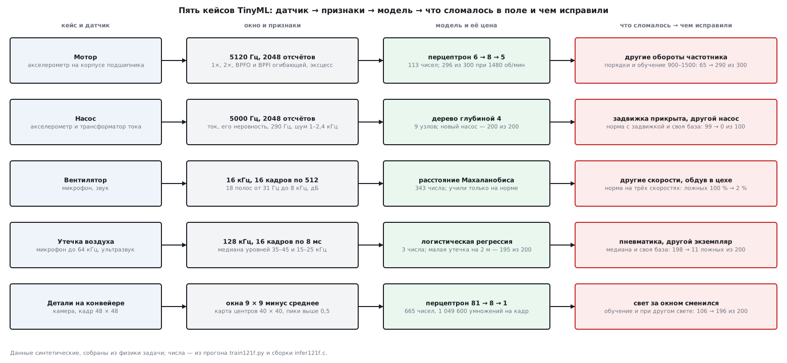
Each case follows one scheme. First the cost of an error: which is dearer, a false alarm or a miss. It sets the threshold and the acceptance measure. Then the sensor and its mounting, the sample rate and window, the features (section 117), the model (sections 116, 116а, 120) and its cost on the F407. Last comes the experiment that usually eats the project: the model is trained, and in the field the speed, the unit, the light or the background changes.
| Case | Sensor, window | Model | Lab acceptance | What broke | After the fix |
|---|---|---|---|---|---|
| Motor | accelerometer, 5120 Hz, 2048 | perceptron 6 → 8 → 5 | 296 of 300 | drive at 900…1000 rpm: 65 of 300 | 290 of 300 |
| Pump | vibration and current, 5000 Hz, 2048 | tree, 9 nodes | 395 of 400 | throttled valve: 99 "cavitations" of 100 | 0 of 100 |
| Fan | microphone, 16 kHz, 8192 | Mahalanobis, 343 numbers | AUC 0.925 | air blowing in the shop: 564 alarms of 600 | 2 of 600 |
| Leak | ultrasound, 128 kHz, 16 × 1024 | logistic, 3 numbers | 156 of 200 found | pneumatics: 198 alarms of 200 | 11 of 200 |
| Parts | camera, 48 × 48 | perceptron 81 → 8 → 1 | 200 of 200 frames | other light: 106 of 200 | 196 of 200 |
All features and models are repeated in C. On the held-out windows C and Python answered the same: motor 100 of 100, pump 60 of 60, fan 60 of 60, leak 60 of 60, parts 60 frames of 60; the motor, pump and fan features differ by at most 3.2·10⁻⁵ relative, the leak levels by 8.2·10⁻⁵ dB, the parts map by 3.8·10⁻⁶.
121д.2 Motor: unbalance, misalignment and the bearing from vibration
Task. An induction motor, 1480 rpm, on a variable-frequency drive. Five states: normal, unbalance, misalignment, outer-race and inner-race bearing defect. A false alarm costs a technician's trip; a missed bearing costs a breakdown and downtime. So acceptance is the recall for the bearing at a low false alarm rate, not the average accuracy.
Sensor. An accelerometer on the bearing housing, on a flat spot, on a stud or glued. 5120 Hz, a window of 2048 samples — 0.4 s and 2.5 Hz per bin.
Physics. Unbalance raises the 1× peak — the shaft speed; misalignment raises 2×. A race defect gives an impact each time a rolling element passes. The impact rates follow from the bearing geometry: 9 balls of 7.94 mm on a 39.04 mm pitch diameter, zero contact angle,
BPFO = n/2 · fr · (1 − d/D), BPFI = n/2 · fr · (1 + d/D),
that is 3.585 and 5.415 times the shaft speed: at 1480 rpm fr = 24.67 Hz, BPFO = 88.4 Hz, BPFI = 133.6 Hz. The impacts are weak, but each rings the housing resonance — 1800 Hz in the model. So the bearing is sought not in the plain spectrum but in the envelope spectrum: a band-pass filter around the resonance, rectification, a spectrum. The inner race turns with the shaft and passes the load zone once per revolution, so its impacts are modulated at 1×.
Features — six, all as logarithms: the RMS, the 1× and 2× peaks, the BPFO and
BPFI peaks of the envelope spectrum divided by its mean level, and the kurtosis of
the signal in the resonance band. The band is two biquad sections, the
envelope is the absolute value:
    biquad(MOT_BP, g_x, g_y, MOT_N);            /* полоса резонанса корпуса */
    biquad(MOT_BP, g_y, g_y, MOT_N);
    f[3] = peak(g_a, MOT_KO * fr, df, 2) / floor;
    f[4] = peak(g_a, MOT_KI * fr, df, 2) / floor;
Model — a 6 → 8 → 5 perceptron (section 116.6), 113 numbers including scaling.
What broke: speed. The first version was trained at 1480 rpm with the feature frequencies written as numbers. At the same speed: 300 correct of 300. Then the motor was put on the drive at 900…1000 rpm: at 950 rpm fr = 15.83 Hz, BPFO = 56.8 Hz, BPFI = 85.7 Hz, and the features look past the peaks. Correct: 65 of 300 — normal 60 of 60, and of 240 faults only 5 recognised. Features in orders — frequencies from the drive speed — but training still at 1480: 185 of 300. Unbalance is recognised in 12 cases of 60: in the model its amplitude grows as the square of the speed, and at 950 rpm it is 2.4 times smaller than in training. The fix is orders plus training over the whole drive range 900…1500 rpm (600 windows): 296 of 300 at 1480 and 290 of 300 on the drive. The errors at 1480 are 4 normal windows taken for unbalance; all 240 faults are recognised.
What broke: mounting. The sensor was put on the plastic fan cover: the cover cuts everything above a few hundred hertz, and the housing resonance does not reach the sensor. The same model: 213 of 300, the bearing found in 34 cases of 120, and 77 bearing defects called normal. The model is not to blame and cannot be "retrained". A self-check helps: the RMS in the resonance band on a healthy motor with good mounting is at least 10.0 mg (median 10.9 mg), on the cover at most 2.0 mg (median 1.8 mg). A threshold between them lets the device say "check the mounting" instead of "normal". Mounting and calibration — section 118.7.
121д.3 Pump: cavitation and dry running from vibration and current
Task. A centrifugal pump, 2900 rpm, an impeller with 6 vanes: fr = 48.3 Hz, blade pass frequency 290.0 Hz. Three states: normal, cavitation, dry running. A missed dry run destroys the seal; a false alarm stops the line. Acceptance is the recall for both faults and the number of alarms on a long normal recording.
Sensors. An accelerometer on the pump casing and a current transformer on a motor phase, both at 5000 Hz, a window of 2048 samples (0.41 s). The rate is chosen so that one 50 Hz mains period is exactly 100 samples.
Physics. Cavitation is collapsing bubbles: bursty broadband noise in the kilohertz range and an uneven current. Dry running has no load: the current drops and the blade pass frequency almost vanishes.
Features — four: the current relative to nominal, the unevenness of the current — the spread of the RMS over 20 mains periods divided by the mean — the level of the blade pass frequency and the RMS of the noise in the 1–2.4 kHz band, both as logarithms:
for (int b = 0; b < 20; b++) { /* 20 периодов сети по 100 отсчётов */
Model — a tree of depth 4, 9 nodes (section 116.4).
What broke: the valve. The first version was trained on four pumps: normal, cavitation, dry running — 299 correct of 300 on the test. In the field the operator throttled the valve. The pump is healthy, but the current fell and became uneven, and of 100 windows with the throttled valve the model called 99 cavitation and 1 dry running. The "throttled valve" mode was added to training as normal.
What broke: another pump. A new pump stands on another base, its noise and blade pass level are higher: all 50 normal windows are "cavitation". Even with the valve in training — again 50 of 50. The fix is an own baseline: at commissioning the device records 20 normal windows and stores the medians of the two levels, and the tree sees the levels relative to them (section 120.4):
float x[4] = { f[0], f[1], f[2] - base[0], f[3] - base[1] };
Result: 395 of 400 on the test — 5 cavitations called normal — the throttled valve 100 of 100 called normal, the new pump 200 of 200. On a stream of 1000 normal and throttled windows of the new pump — not a single alarm; on a fault stream 198 cavitations of 200 and 200 dry runs of 200 are found.
121д.4 Fan: an anomaly by sound
Task. A fan with 7 blades on a drive: 900, 1200 and 1500 rpm, blade pass frequency 105, 140 and 175 Hz. There are no fault recordings, so the model learns only the normal state (section 120) and alarms when the sound is far from it. A false alarm in sound monitoring is cheaper than at the pump, but with too many of them the device gets switched off.
Sensor. A microphone next to the fan (signal chain — section 121б), 16 kHz, a window of 16 frames of 512 samples — 0.51 s.
Features — 18 bands, from bin 1 to 256, i.e. from 31 Hz to 8 kHz, wider at higher frequencies; the level is the mean power over 16 frames in decibels. The low bands are there for 1×: without them a damaged blade is invisible.
Model — the Mahalanobis distance to normal: the mean of the 18 bands and the inverse covariance matrix, 343 numbers. The threshold is the 99.5th percentile of the distance on a separate normal set.
    for (int i = 0; i < FAN_NB; i++) {
        float r = 0;
        for (int j = 0; j < FAN_NB; j++)
            r += FAN_P[i * FAN_NB + j] * d[j];
        s += d[i] * r;
    }
Three anomalies: a damaged blade (a 1× peak and modulation of the blade pass frequency), a bearing (noise in a band around 4 kHz), rubbing (a click once per revolution).
What broke: speed. The normal state was recorded at 1500 rpm. At 1500: 7 alarms of 200 normal windows; at 1200 and 900: 200 of 200 — another speed is another spectrum, and for the model that is an anomaly. AUC over all speeds is 0.608. The fix is the normal state at all three speeds: 12 alarms of 600, 156 damaged blades of 200 found, 180 bearings and 108 rubbing cases, AUC 0.925.
What broke: background. Compressed-air blowing was switched on in the shop — a hiss at 2–8 kHz. Alarms: 564 of 600 normal windows. Recordings with the blowing were added to the normal state: 0 alarms of 600 without blowing and 2 of 600 with it. But the threshold rose from 19.61 to 38.89, and the model went blind where the air hisses: 37 blades of 200, 129 bearings and 42 rubbing cases found, and with the blowing on — 51, 30 and 27. That is the honest price: a microphone hears everything around. For a bearing in a noisy shop a sensor on the housing is better, as in 121д.2; the microphone stays where the background is known.
121д.5 Compressed-air leak by ultrasound
Task. Walking a pipeline with a hand-held device, or a fixed sensor at a section. A leak is turbulent noise, in the model with a maximum around 40 kHz, where the shop noise has already died out. A false alarm is a needless search along the line; a miss costs compressor energy but is not a breakdown. Acceptance is the distance at which a leak of a given size is found.
Sensor. A microphone with a bandwidth up to 64 kHz, 128 kHz sampling, a frame of 1024 samples — 125 Hz per bin and 8 ms, window of 16 frames. Levels are taken in the 35–45 kHz band (leak) and the 15–25 kHz band (shop noise). The model includes 1/r spreading and 1.3 dB/m absorption in air.
What broke: pneumatics. First version: the mean level over the frames, logistic regression, training on one sensor unit with no interference. On the test: 0 alarms of 200 and 156 leaks of 200. The shop has pneumatic cylinders: the exhaust gives ultrasound in 1–4 frames of 16, and the alarms are 198 of 200. A leak hisses all the time, an exhaust briefly; the mean does not tell them apart, the median over 16 frames does:
    f[0] = median16(u) - base[0];
    f[1] = median16(m) - base[1];
What broke: the unit. Microphone sensitivity varies; ±6 dB in the model. For a unit at +4…+6 dB the first version gives 69 alarms of 200, for a unit at −6…−4 dB it finds 133 leaks of 200. The fix is an own baseline: at installation the device records 10 quiet windows and takes the features relative to them. Training uses 24 units and the pneumatics, 384 windows.
Result: 0 alarms of 200 without interference and 11 of 200 with pneumatics; 124 small leaks of 200 and 198 medium ones found at 1–5 m. Weak points remain: the sensitive unit gives 27 alarms of 200 — above the amplifier noise the shop noise itself rises, and it wanders from window to window; for the unit at −6…−4 dB 70 small leaks of 200 are found. Range — out of 200:
| Distance | 1 m | 2 m | 3 m | 4 m | 6 m |
|---|---|---|---|---|---|
| Small leak | 200 | 195 | 101 | 46 | 10 |
| Medium, 10 dB louder | 200 | 200 | 200 | 195 | 109 |
Ultrasound is a short-range tool: a small leak is reliably found within 2 m, and that belongs in the walk-around instructions.
121д.6 Parts on a conveyor: a centre detector
Task. A camera above the belt counts the parts in the frame. A count error either way spoils the accounting; acceptance is the share of frames with an exact count and the share of parts found. Presence of a person in a zone is solved the same way — by detection in the frame; a large detector on a camera is section 121в.
Sensor and frame. A grey 48 × 48 frame after downscaling. The parts are bright discs of radius 3–4.5 pixels, 0 to 6 per frame, often touching: of 200 test frames 115 contain touching parts.
Threshold and blobs did not cope. Threshold 122.7 and connected regions, as
find_blobs in section 121а: under normal light an exact count in 178 frames of
200 and 589 parts of 613 — touching parts merge into one blob. When the light
changed — darker, a brightness slope from the window, glare — 51 frames of 200 and
152 parts of 565.
Centre detector. A small network looks at a 9 × 9 window around every point and answers how much this point is the centre of a part. It is a 9 × 9 convolution with 8 filters, ReLU and a 1 × 1 convolution. The input is the window minus its mean, divided by the frame RMS: so the overall level and slope of the light are removed before the network. The training target is a Gaussian spot at each part centre; the answer is a 40 × 40 map, parts are peaks above 0.5.
            for (int i = 0; i < DET_P * DET_P; i++)
                z[i] = (z[i] - pm) * inv;
665 numbers and 1049600 multiplications per frame.
What broke: light. The detector trained under normal light is flawless under it: 200 frames of 200, all 613 parts. Under other light: 106 frames of 200 — 562 parts of 565 found, but 777 peaks: glare and shadow edges give false centres. The fix is half of the training frames under changed light: 196 frames of 200, 561 parts of 565 with 563 peaks, and under normal light still 200 of 200. Light on site always changes; training frames are shot morning, noon and evening or distorted in software.
Cost on the F407. Functions from the armclang object file:
| Case | Feature and model code | Tables outside code | Model numbers |
|---|---|---|---|
| Motor | 3660 + 1688 bytes | — | 113 |
| Pump | 1896 + 128 bytes | 72 bytes | 9 nodes |
| Fan | 380 + 592 bytes | 1372 bytes | 343 |
| Leak | 1746 + 52 bytes | — | 3 |
| Parts | 3106 + 390 bytes | 2592 bytes | 665 |
The shared spectrum with the FFT is another 1748 bytes. The buffers are shared by all cases: the complex FFT buffer for 2048 points is 16384 bytes, the window and the filter output 8192 each, the spectrum 4100; 37896 bytes of RAM in total. The input window is separate: 8 KB of float for the motor, 64 KB for 16 leak frames, so on the device the leak frames are processed as they arrive and only 32 levels are kept.
121д.7 Pitfalls
100 % in the lab, a third in the field. The features are tied to frequencies at one speed. Frequencies are computed in orders from the drive speed, and training covers the whole range: for the motor 65 → 290 of 300.
The model "does not see" the bearing. The sensor is on the cover or on paint: high frequencies do not reach it. The model is not to blame; the device must check the resonance band level and complain about the mounting.
A healthy pump in alarm. Training lacked a mode that is common in the field — the throttled valve. Operating modes are collected before training, from the operator and the process engineer, not after the first false alarm.
The second device lies, the first does not. Another unit: another base, another microphone. Absolute levels are replaced by levels relative to an own baseline taken at commissioning.
Background added to normal — and misses. A model of normal stretches the threshold over everything it was shown: the blowing removed 562 false alarms, but also half of the detections.
A mean over the window catches short interference. A pneumatic exhaust in 4 frames of 16 raises the mean; the median does not see it.
The detector counts glare. There was one lighting condition in training. Training frames cover all lighting conditions, and the input has the local mean removed.
C and Python compared on one window. An error in a bin index or in the weight order does not show everywhere. Compare on dozens of windows of all classes and modes: here 340 windows and frames.
121д.8 Summary
- Motor: BPFO = 3.585·fr and BPFI = 5.415·fr from the bearing geometry, the envelope in the resonance band; frequencies as numbers — 65 of 300 on the drive, orders and the whole range — 290 of 300.
- Mounting on the cover: 34 bearings of 120; the resonance band level of 10.9 mg against 1.8 mg is a self-check feature.
- Pump: the throttled valve gave 99 false cavitations of 100, another pump 50 of 50; the mode in training and an own baseline — 0 and 200 correct of 200.
- Fan: normal at one speed — 200 alarms of 200 at the others; at three — 12 of 600 and AUC 0.925; background in the normal set removes alarms, but also detections.
- Leak: the median over frames — 198 → 11 false alarms of 200 with pneumatics; a small leak is found in 195 cases of 200 at 2 m and in 46 at 4 m.
- Parts: threshold and blobs — 178 and 51 frames of 200; the centre detector trained under varied light — 200 and 196.
- All five cases are repeated in C: the answers matched Python on all 340 windows and frames; feature and model code is 972 to 5348 bytes per case on the F407.
Full sources
infer121f.c — features and models of the five cases in C, float, with parameters from model121f.h.
/* Раздел 121д: пять промышленных кейсов — признаки и модели на Cortex-M4F во float.
 * Параметры — из model121f.h (выгрузил train121f.py). Каждый кейс — функция признаков
 * из сырого окна датчика и функция ответа модели:
 *   мотор   — 6 признаков вибрации, перцептрон 6 → 8 → 5;
 *   насос   — 4 признака вибрации и тока, дерево решений;
 *   вентилятор — 18 полос звука, расстояние Махаланобиса до нормы;
 *   утечка  — 2 уровня ультразвука к своей базе, логистическая регрессия;
 *   детали  — карта центров по окнам 9 × 9, перцептрон 81 → 8 → 1, счёт пиков.
 * На компьютере main читает test121f.bin и сверяет признаки и ответы с Python
 * (-DML_HOST). Проверка — _verify/ml121f_check.py. */
#include <math.h>

#include "model121f.h"

#define NMAX 2048
static float g_re[2 * NMAX];                    /* комплексный буфер БПФ */
static float g_a[NMAX / 2 + 1];                 /* амплитудный спектр */
static float g_x[NMAX], g_y[NMAX];              /* окно и выход фильтра */

/* БПФ по основанию 2 на месте: re, im чередуются */
static void fft(float *d, int n)
{
    for (int i = 1, j = 0; i < n; i++) {
        int b = n >> 1;
        for (; j & b; b >>= 1)
            j ^= b;
        j ^= b;
        if (i < j) {
            float t = d[2 * i]; d[2 * i] = d[2 * j]; d[2 * j] = t;
            t = d[2 * i + 1]; d[2 * i + 1] = d[2 * j + 1]; d[2 * j + 1] = t;
        }
    }
    for (int len = 2; len <= n; len <<= 1) {
        for (int k = 0; k < len / 2; k++) {
            float wr = cosf(-6.28318531f * k / len), wi = sinf(-6.28318531f * k / len);
            for (int i = k; i < n; i += len) {
                int j = i + len / 2;
                float xr = d[2 * j] * wr - d[2 * j + 1] * wi, xi = d[2 * j] * wi + d[2 * j + 1] * wr;
                d[2 * j] = d[2 * i] - xr;
                d[2 * j + 1] = d[2 * i + 1] - xi;
                d[2 * i] += xr;
                d[2 * i + 1] += xi;
            }
        }
    }
}

/* Амплитудный спектр с окном Ханна: синус амплитуды A даёт пик A */
static void amp_spec(const float *x, int n, float *a)
{
    for (int i = 0; i < n; i++) {
        g_re[2 * i] = x[i] * (0.5f - 0.5f * cosf(6.28318531f * i / n));
        g_re[2 * i + 1] = 0.0f;
    }
    fft(g_re, n);
    for (int k = 0; k <= n / 2; k++)
        a[k] = sqrtf(g_re[2 * k] * g_re[2 * k] + g_re[2 * k + 1] * g_re[2 * k + 1]) * 4.0f / n;
}

/* Звено второго порядка, прямая форма I */
static void biquad(const float c[5], const float *x, float *y, int n)
{
    float x1 = 0, x2 = 0, y1 = 0, y2 = 0;
    for (int i = 0; i < n; i++) {
        float v = c[0] * x[i] + c[1] * x1 + c[2] * x2 - c[3] * y1 - c[4] * y2;
        x2 = x1; x1 = x[i]; y2 = y1; y1 = v;
        y[i] = v;
    }
}

static float peak(const float *a, float f, float df, int w)
{
    int k = (int)(f / df + 0.5f);
    float m = a[k - w];
    for (int i = k - w + 1; i <= k + w; i++)
        if (a[i] > m)
            m = a[i];
    return m;
}

static float mean(const float *x, int n)
{
    float s = 0;
    for (int i = 0; i < n; i++)
        s += x[i];
    return s / n;
}

/* ── 1. Мотор: 1×, 2×, BPFO и BPFI огибающей, эксцесс; fr — от частотника ── */
void mot_features(const float *x, float fr, float f[6])
{
    const float df = MOT_FS / MOT_N;
    float m = mean(x, MOT_N), s2 = 0, s4 = 0, floor = 0;
    for (int i = 0; i < MOT_N; i++) {
        g_x[i] = x[i] - m;
        s2 += g_x[i] * g_x[i];
    }
    f[0] = sqrtf(s2 / MOT_N);
    amp_spec(g_x, MOT_N, g_a);
    f[1] = peak(g_a, fr, df, 1);
    f[2] = peak(g_a, 2 * fr, df, 1);
    biquad(MOT_BP, g_x, g_y, MOT_N);            /* полоса резонанса корпуса */
    biquad(MOT_BP, g_y, g_y, MOT_N);
    s2 = 0;
    for (int i = 0; i < MOT_N; i++) {
        float v = g_y[i] * g_y[i];
        s2 += v;
        s4 += v * v;
        g_y[i] = fabsf(g_y[i]);                 /* огибающая: выпрямление */
    }
    f[5] = s4 / MOT_N / ((s2 / MOT_N) * (s2 / MOT_N));
    m = mean(g_y, MOT_N);
    for (int i = 0; i < MOT_N; i++)
        g_y[i] -= m;
    amp_spec(g_y, MOT_N, g_a);
    for (int k = 4; k < 200; k++)
        floor += g_a[k];
    floor /= 196;
    f[3] = peak(g_a, MOT_KO * fr, df, 2) / floor;
    f[4] = peak(g_a, MOT_KI * fr, df, 2) / floor;
    for (int i = 0; i < 6; i++)
        f[i] = log10f(f[i]);
}

int mot_classify(const float f[6])
{
    float h[8], best = -3.4e38f;
    int c = 0;
    for (int j = 0; j < 8; j++) {
        float a = MOT_B1[j];
        for (int i = 0; i < 6; i++)
            a += (f[i] - MOT_MU[i]) / MOT_SD[i] * MOT_W1[i * 8 + j];
        h[j] = a > 0 ? a : 0;
    }
    for (int k = 0; k < 5; k++) {
        float a = MOT_B2[k];
        for (int j = 0; j < 8; j++)
            a += h[j] * MOT_W2[j * 5 + k];
        if (a > best) {
            best = a;
            c = k;
        }
    }
    return c;
}

/* ── 2. Насос: ток к номиналу, неровность тока, лопастная частота, шум 1–2,4 кГц ── */
void pump_features(const float *v, const float *cur, float f[4])
{
    const float df = PUMP_FS / PUMP_N;
    float s = 0, bm = 0, bs = 0, blk[20];
    for (int i = 0; i < PUMP_N; i++)
        s += cur[i] * cur[i];
    f[0] = sqrtf(s / PUMP_N) / PUMP_INOM;
    for (int b = 0; b < 20; b++) {              /* 20 периодов сети по 100 отсчётов */
        float q = 0;
        for (int i = 0; i < 100; i++)
            q += cur[b * 100 + i] * cur[b * 100 + i];
        blk[b] = sqrtf(q / 100);
        bm += blk[b];
    }
    bm /= 20;
    for (int b = 0; b < 20; b++)
        bs += (blk[b] - bm) * (blk[b] - bm);
    f[1] = sqrtf(bs / 20) / bm;
    float m = mean(v, PUMP_N);
    for (int i = 0; i < PUMP_N; i++)
        g_x[i] = v[i] - m;
    amp_spec(g_x, PUMP_N, g_a);
    f[2] = log10f(peak(g_a, PUMP_VANES * 2900 / 60.0f, df, 3));
    s = 0;
    for (int k = (int)(1000 / df + 0.5f); k < (int)(2400 / df + 0.5f); k++)
        s += g_a[k] * g_a[k];
    f[3] = log10f(sqrtf(s / 2));
}

/* base — медианы lg A_bpf и lg шума этого насоса по 20 окнам при пуске */
int pump_classify(const float f[4], const float base[2])
{
    float x[4] = { f[0], f[1], f[2] - base[0], f[3] - base[1] };
    int n = 0;
    while (PUMP_LEFT[n] >= 0)
        n = x[PUMP_FEAT[n]] <= PUMP_THR[n] ? PUMP_LEFT[n] : PUMP_RIGHT[n];
    return PUMP_CLASS[n];
}

/* ── 3. Вентилятор: 18 полос по 16 кадрам 512, расстояние до нормы ── */
void fan_features(const float *x, float f[FAN_NB])
{
    static float p[FAN_FR / 2 + 1];
    for (int k = 0; k <= FAN_FR / 2; k++)
        p[k] = 0;
    for (int fr = 0; fr < FAN_NF; fr++) {
        amp_spec(x + fr * FAN_FR, FAN_FR, g_a);
        for (int k = 0; k <= FAN_FR / 2; k++)
            p[k] += g_a[k] * g_a[k] / FAN_NF;
    }
    for (int j = 0; j < FAN_NB; j++) {
        float e = 0;
        for (int k = FAN_KB[j]; k < FAN_KB[j + 1]; k++)
            e += p[k];
        f[j] = 10.0f * log10f(e + 1e-12f);
    }
}

float fan_score(const float f[FAN_NB])
{
    float d[FAN_NB], s = 0;
    for (int i = 0; i < FAN_NB; i++)
        d[i] = f[i] - FAN_MU[i];
    for (int i = 0; i < FAN_NB; i++) {
        float r = 0;
        for (int j = 0; j < FAN_NB; j++)
            r += FAN_P[i * FAN_NB + j] * d[j];
        s += d[i] * r;
    }
    return s;
}

int fan_anomaly(const float f[FAN_NB])
{
    return fan_score(f) > FAN_THR;
}

/* ── 4. Утечка: медиана по 16 кадрам уровней 35–45 и 15–25 кГц минус своя база ── */
static float band_db(int k0, int k1)
{
    float e = 0;
    for (int k = k0; k < k1; k++)
        e += g_a[k] * g_a[k];
    return 10.0f * log10f(e / 2 + 1e-15f);
}

static float median16(float *v)
{
    for (int i = 1; i < 16; i++)                /* вставками: 16 чисел */
        for (int j = i; j > 0 && v[j - 1] > v[j]; j--) {
            float t = v[j]; v[j] = v[j - 1]; v[j - 1] = t;
        }
    return 0.5f * (v[7] + v[8]);
}

void leak_features(const float *x, const float base[2], float f[2])
{
    float u[LEAK_NF], m[LEAK_NF];
    for (int fr = 0; fr < LEAK_NF; fr++) {
        amp_spec(x + fr * LEAK_FR, LEAK_FR, g_a);
        u[fr] = band_db(LEAK_US0, LEAK_US1);
        m[fr] = band_db(LEAK_MID0, LEAK_MID1);
    }
    f[0] = median16(u) - base[0];
    f[1] = median16(m) - base[1];
}

int leak_detect(const float f[2])
{
    return LEAK_W[0] * f[0] + LEAK_W[1] * f[1] + LEAK_B > 0.0f;
}

/* ── 5. Детали на конвейере: карта центров 40 × 40 и пики ── */
#define DET_R (DET_P / 2)
#define DET_O (DET_W - 2 * DET_R)

void det_heatmap(const float *img, float *hm)
{
    float s = 0, s2 = 0, z[DET_P * DET_P];
    for (int i = 0; i < DET_W * DET_W; i++)
        s += img[i];
    s /= DET_W * DET_W;
    for (int i = 0; i < DET_W * DET_W; i++)
        s2 += (img[i] - s) * (img[i] - s);
    float inv = 1.0f / (sqrtf(s2 / (DET_W * DET_W)) + 1.0f);
    for (int y = 0; y < DET_O; y++)
        for (int x = 0; x < DET_O; x++) {
            float pm = 0, out = DET_B2[0];
            for (int dy = 0; dy < DET_P; dy++)
                for (int dx = 0; dx < DET_P; dx++)
                    pm += z[dy * DET_P + dx] = img[(y + dy) * DET_W + x + dx];
            pm /= DET_P * DET_P;
            for (int i = 0; i < DET_P * DET_P; i++)
                z[i] = (z[i] - pm) * inv;
            for (int j = 0; j < DET_HID; j++) {
                float a = DET_B1[j];
                for (int i = 0; i < DET_P * DET_P; i++)
                    a += z[i] * DET_W1[i * DET_HID + j];
                out += (a > 0 ? a : 0) * DET_W2[j];
            }
            hm[y * DET_O + x] = out;
        }
}

int det_count(const float *hm)
{
    int n = 0;
    for (int y = 0; y < DET_O; y++)
        for (int x = 0; x < DET_O; x++) {
            float v = hm[y * DET_O + x];
            int top = v > 0.5f;
            for (int dy = -1; dy <= 1 && top; dy++)
                for (int dx = -1; dx <= 1; dx++) {
                    int yy = y + dy, xx = x + dx;
                    if (yy >= 0 && yy < DET_O && xx >= 0 && xx < DET_O && hm[yy * DET_O + xx] > v)
                        top = 0;
                }
            n += top;
        }
    return n;
}

#ifdef ML_HOST
#include <stdio.h>
#include <stdlib.h>

static FILE *fb;
static void rd(void *p, size_t n)
{
    if (fread(p, 1, n, fb) != n) {
        printf("short read\n");
        exit(1);
    }
}

static float rel(float a, float b)
{
    float d = fabsf(a - b), m = fabsf(b) > 1e-3f ? fabsf(b) : 1e-3f;
    return d / m;
}

int main(int argc, char **argv)
{
    static float x[LEAK_FR * LEAK_NF], cur[PUMP_N], hm[DET_O * DET_O], hp[DET_O * DET_O];
    float f[FAN_NB], fp[FAN_NB], e, fr, base[2], sp;
    int n, cls, same, i, k;
    fb = fopen(argc > 1 ? argv[1] : "test121f.bin", "rb");
    if (!fb)
        return 1;
    rd(&n, 4);                                     /* мотор */
    for (i = same = 0, e = 0; i < n; i++) {
        rd(&fr, 4); rd(x, 4 * MOT_N); rd(fp, 4 * 6); rd(&cls, 4);
        mot_features(x, fr, f);
        for (k = 0; k < 6; k++)
            e = fmaxf(e, rel(f[k], fp[k]));
        same += mot_classify(f) == cls;
    }
    printf("mot=%d,%d,%.1e\n", same, n, e);
    rd(&n, 4); rd(base, 8);                        /* насос */
    for (i = same = 0, e = 0; i < n; i++) {
        rd(x, 4 * PUMP_N); rd(cur, 4 * PUMP_N); rd(fp, 4 * 4); rd(&cls, 4);
        pump_features(x, cur, f);
        for (k = 0; k < 4; k++)
            e = fmaxf(e, rel(f[k], fp[k]));
        same += pump_classify(f, base) == cls;
    }
    printf("pump=%d,%d,%.1e\n", same, n, e);
    rd(&n, 4);                                     /* вентилятор */
    for (i = same = 0, e = 0; i < n; i++) {
        rd(x, 4 * FAN_FR * FAN_NF); rd(fp, 4 * FAN_NB); rd(&sp, 4); rd(&cls, 4);
        fan_features(x, f);
        for (k = 0; k < FAN_NB; k++)
            e = fmaxf(e, rel(f[k], fp[k]));
        e = fmaxf(e, rel(fan_score(f), sp));
        same += fan_anomaly(f) == cls;
    }
    printf("fan=%d,%d,%.1e\n", same, n, e);
    rd(&n, 4);                                     /* утечка */
    for (i = same = 0, e = 0; i < n; i++) {
        rd(base, 8); rd(x, 4 * LEAK_FR * LEAK_NF); rd(fp, 4 * 2); rd(&cls, 4);
        leak_features(x, base, f);
        for (k = 0; k < 2; k++)
            e = fmaxf(e, fabsf(f[k] - fp[k]));      /* дБ: абсолютная разница */
        same += leak_detect(f) == cls;
    }
    printf("leak=%d,%d,%.1e\n", same, n, e);
    rd(&n, 4);                                     /* детали */
    for (i = same = 0, e = 0; i < n; i++) {
        rd(x, 4 * DET_W * DET_W); rd(hp, 4 * DET_O * DET_O); rd(&cls, 4);
        det_heatmap(x, hm);
        for (k = 0; k < DET_O * DET_O; k++)
            e = fmaxf(e, fabsf(hm[k] - hp[k]));
        same += det_count(hm) == cls;
    }
    printf("det=%d,%d,%.1e\n", same, n, e);
    printf("done=1\n");
    fclose(fb);
    return 0;
}
#endif
Next: section 121е "A TinyML course project: your own model for a task from scratch to the firmware — gesture recognition with a wristband on the STM32F407" — all the steps of part XIV in a row on one task: the collection firmware, recordings of 24 people, exploration and cleaning, two models, int8, the recognition firmware with smoothing and the final budget.