 Embedded HandbookApps
118. Training a small model in a container
In section 116 the models learned from tidy points, in section 117 the features were computed from signal windows. Here everything is brought together and moved closer to what happens at a factory: the data come as recordings — one run of one motor with one sensor mounting — dozens of similar windows are cut from a recording, the classes are not equal in size, and every sensor has its own sensitivity. The section shows how to split such data so that the estimate does not lie, how to choose the size of the model, what to do with a rare class and how to carry the weights into the firmware so that C answers exactly like Python.
Training runs in the stm-ml:1 image — numpy 2.3.3 and scikit-learn 1.7.2 —
and repeats verbatim: the same weights, the same numbers down to the last digit.
Approaches are section 116, features are section 117.
Terms used in the documentation
Term Meaning recording, session one run of one object labeling, annotation assigning a class to a recording train / validation / test split dividing data into training, tuning and final testing data leakage information about the test set getting into training group k-fold cross-validation by groups (recordings) hyperparameter a setting such as model size or tree depth confusion matrix a table of true classes against the model's answers class imbalance some classes have few examples class weight the weight of a class in training recall / precision share of defects found / share of alarms that are real false alarm an alarm with no real defect calibration calibrating the sensor on site reproducible build a build that gives the same result every time literal pool constants placed next to the code
118.1 Recordings, not points
The data set of this section is 1800 windows from 90 recordings: 30 recordings per state (normal, imbalance, bearing), 20 windows per recording. Each recording has its own rotation frequency, amplitudes and sensor mounting sensitivity; the windows of one recording differ only in phase and noise. The features of a window are the four numbers from section 117: RMS, peak frequency, crest factor and the share of energy in the 100–248 Hz band.
The main property of such data: the windows of one recording are almost identical. A model that has seen 14 windows of a recording will recognize the fifteenth not because it understood imbalance, but because it memorized this motor. On the device, however, it will meet a motor that was not in the training data.
118.2 Labeling
The label is assigned to a whole recording: a motor with imbalance, a bearing due for replacement, a motor after repair — normal. The most reliable way is to label by what is established outside the signal: a repair report, an inspection, a test rig with a known defect. Labeling "by eye from the spectrum" teaches the model to repeat the eye of the labeler, not to see the defect.
Recordings are stored together with metadata: which motor, which sensor, how it is mounted, what sampling rate and the version of the firmware that made the recording. Without them you cannot figure out why the model makes mistakes, and you cannot split the data by recordings.
118.3 Splitting: leakage between windows of one recording
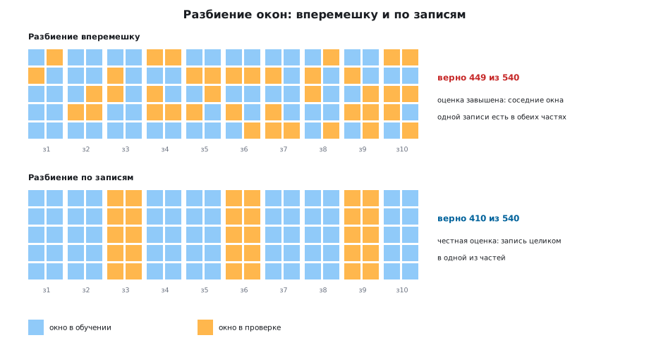
Two ways to set aside 30 % of the data for testing. Shuffled — windows are picked at random, and almost every recording has some windows in training and some in the test:
tr, te = train_test_split(np.arange(len(y)), test_size=0.3, random_state=118, stratify=y)
By recordings — whole recordings go to the test:
rtr, rte = train_test_split(recs, test_size=0.3, random_state=118, stratify=recs // 1000)
mtr, mte = np.isin(g, rtr), np.isin(g, rte)
One and the same model — a 4 → 4 → 3 perceptron — is right in the first case in 449 out of 540 (83.1 %), in the second in 410 out of 540 (75.9 %). The difference is what the model learned about specific motors. It is even more visible with a model that only remembers, the nearest neighbour: 460 with a random split and 444 with a split by recordings. The rule is simple: the test must not contain a single window of a recording whose windows were in training. The same goes for the overlapping windows from section 117: neighbouring overlapping windows are almost copies.
118.4 Normalization is part of the model
The perceptron learns on features brought to zero mean and unit spread. The mean and spread are computed only from the training recordings — otherwise the test leaks into training here as well:
m, s = X[mtr].mean(axis=0), X[mtr].std(axis=0)
mlp = mk().fit((X[mtr] - m) / s, y[mtr])
These eight numbers are as much a part of the model as the weights. They go
into the firmware together with the weights (the MU and SD arrays), and the device normalizes
the features with them, not with its own. Forgetting them is the most common reason why
a model that worked perfectly in Python gives the same answer every time on the board.
118.5 Model size: cross-validation by recordings
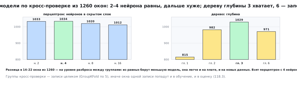
How many neurons in the hidden layer and how deep the tree should be is decided not by the test part — it is touched only once, at the end. The training recordings are split into 5 groups; the model learns on four and answers on the fifth, in turn. The groups are whole recordings:
gkf = GroupKFold(n_splits=5)
for a, b in gkf.split(X[mtr], y[mtr], g[mtr]):
| Neurons in the hidden layer | 2 | 4 | 8 | 16 |
|---|---|---|---|---|
| Correct out of 1260 | 1033 | 1034 | 1020 | 1012 |
| Tree depth | 1 | 2 | 3 | 6 |
|---|---|---|---|---|
| Correct out of 1260 | 815 | 982 | 1029 | 971 |
For the perceptron, 2 and 4 neurons cannot be told apart, and beyond that it gets worse: the extra neurons learn the quirks of the training motors. For the tree, depth 1 cannot cope — three classes cannot be separated with one question — and depth 6 already memorizes. The perceptron with 4 neurons is chosen. A difference of 14–22 windows out of 1260 is at the level of the spread between groups, so among equals you pick the smaller model: it is lighter both on the board and on new data.
118.6 Confusion matrix of the final model
The final perceptron is trained on all training recordings and tested once on the held-out ones — 27 recordings, 540 windows:
| True / model's answer | normal | imbalance | bearing |
|---|---|---|---|
| Normal | 70 | 110 | 0 |
| Imbalance | 20 | 160 | 0 |
| Bearing | 0 | 0 | 180 |
The bearing is error-free: it is given away by the band energy, the feature from section 117. Normal, however, is taken for imbalance in most windows. The reason is not the model: normal and imbalance differ only in the strength of vibration, and the strength the sensor sees depends on the mounting. A tight mounting on a normal motor gives the same RMS as a loose mounting on a motor with imbalance. No model size will fix this — you need different data.
118.7 Calibrating the mounting
The sensitivity of the mounting is measured when the sensor is installed: a known tap or a reference vibration rig, and the RMS is divided by the coefficient found. In the experiment this is one line:
Xc[:, 0] /= gain_w
The same perceptron after calibration gets 481 out of 540: normal is recognized in 168 windows out of 180 instead of 70. Imbalance is recognized less often — in 133 windows out of 180 instead of 160 — because imbalances themselves vary in strength, and the weak ones stray into the territory of normal; that is now a question of the alarm threshold, not of the data. The lesson of section 116 repeats: a good feature and honest data give more than the choice of model.
118.8 A rare class and class weights
At a factory there are many healthy motors and few defective ones. In the experiment every twentieth bearing window is kept: there are 21 bearing windows out of 861 in training. A tree of depth 2 counts all errors equally, and it pays for it to almost always answer "not a bearing": without weights it found 60 bearings out of 180, with class weights 180, and false alarms — 0. The weight of a class is inversely proportional to its share, and every error on the rare class costs more:
q = DecisionTreeClassifier(max_depth=2, random_state=118, class_weight=cw).fit(X[thin], y[thin]).predict(X[mte])
For a device two quantities matter separately: recall — what share of defects it found, and precision — what share of alarms are real. Here "precision" is the strict term; in sections 116 and 119 the word "accuracy" was used for short for the share of correct answers. A single overall share of correct answers hides both quantities: a model that misses every bearing would still be right in two cases out of three here.
118.9 Into the firmware: header, cross-check, reproducibility
Training writes model118.h: the normalization, the weights and the held-out windows
with the answers of scikit-learn. The C inference is 43 numbers and 28 multiplications; the hidden layer:
for (i = 0; i < N_FEAT; i++)
    z[i] = (f[i] - MU[i]) / SD[i];
for (j = 0; j < N_HIDDEN; j++) {
    float s = B1[j];
    for (i = 0; i < N_FEAT; i++)
        s += z[i] * W1[i * N_HIDDEN + j];
    h[j] = s > 0.0f ? s : 0.0f;                 /* ReLU */
}
Built with -DML_HOST on a PC, the same file runs all
held-out windows: the answers of C and scikit-learn matched in all 540 windows.
Such a cross-check is a mandatory step: a mixed-up order of the weights (in
scikit-learn the matrix is "input × neuron"), a forgotten normalization or
the wrong number type show up at once, not on site.
armclang built the inference into 548 bytes of code on the F407 and 882 on the F103 — the F103 has no FPU, and floating-point addition and multiplication call the library. The compiler unrolled both loops completely: the 172 bytes of weights became literals, and there are 352 bytes of literals in the code — the weights and constants the compiler derived from them. For a model of a few dozen numbers this is the fastest way; for thousands of weights the loops remain, and the weights sit as an array in flash.
Reproducibility: an image with pinned versions, a generator seed
at every random step (random_state=118), and retraining
must produce the same model118.h byte for byte. If the weights changed
but the data did not, the library changed, and you must notice it before flashing.
118.10 Pitfalls
99 % in Python, nonsense on site. Windows of one recording were both in training and in the test. Split by recordings, with groups in cross-validation too.
On the board the model gives the same answer every time. The mean and spread of the normalization were not carried over, or the features on the board are computed differently than in training. Normalization goes into the header, features use one code base (section 117).
The share of correct answers is high, but defects are missed. A rare class: it pays the model not to notice it. Class weights and recall for each class.
One motor is normal, the next one is imbalance, though both are healthy. Different mounting sensitivity. Calibration at installation.
Retrained — and the weights are different. Versions or the seed are not pinned.
A container with versions, random_state, comparing the header with the previous one.
The model was chosen by the test part. After that it is no longer a test part. Tuning by cross-validation, testing once at the end.
118.11 Summary
- 1800 windows from 90 recordings: a shuffled split gave 83.1 %, by recordings 75.9 %; the honest figure is the second.
- The model size is chosen by cross-validation by recordings: 4 neurons, a tree of depth 3.
- Normalization is part of the model and goes into the firmware together with the weights.
- Normal is told from imbalance not by the model but by mounting calibration: 410 → 481 out of 540.
- A rare class needs class weights: 180 bearings out of 180 found instead of 60.
- The C inference is checked against Python on all held-out windows; the 4 → 4 → 3 perceptron is 548 bytes of code on the F407.
Full sources
train118.py — training the perceptron from recordings to weights in a header for the firmware.
# -*- coding: utf-8 -*-
"""Раздел 118: обучение маленькой модели — от записей к весам в прошивке.

Запуск — в образе stm-ml:1:  python train118.py <каталог_вывода>

Данные устроены как настоящие: запись — один прогон одного мотора, у неё свои
амплитуда и частота; из записи нарезано 20 окон, похожих друг на друга.
Признаки окна те же, что в разделе 117 (СКЗ, частота пика, пик-фактор, доля
энергии в полосе 100–248 Гц), посчитаны теми же формулами (117 сверил их
с CMSIS-DSP). Опыты:
  • утечка: случайное разбиение окон против разбиения по записям;
  • подбор гиперпараметров кросс-проверкой по группам записей;
  • редкий класс: подшипников в 20 раз меньше — точность против полноты;
  • выгрузка перцептрона 4 → 4 → 3 в model118.h для infer118.c и сверка с C.
Сводка — в summary118.txt."""
import sys

import numpy as np
from sklearn.metrics import confusion_matrix
from sklearn.model_selection import GroupKFold, train_test_split
from sklearn.neural_network import MLPClassifier
from sklearn.tree import DecisionTreeClassifier

OUT = sys.argv[1] if len(sys.argv) > 1 else "."
rng = np.random.RandomState(118)
N, FS, WPR = 256, 1024.0, 20                      # отсчётов в окне, Гц, окон на запись
t = np.arange(N) / FS
hann = 0.5 * (1 - np.cos(2 * np.pi * np.arange(N) / N))


def feats(x):
    y = x - x.mean()
    rms = np.sqrt((y ** 2).mean())
    crest = np.abs(y).max() / rms
    m = np.abs(np.fft.rfft(y * hann))[:N // 2]
    m[0] = 0
    k = int(m.argmax())
    a, b, c = m[k - 1], m[k], m[k + 1]
    peak = (k + 0.5 * (a - c) / (a - 2 * b + c)) * FS / N
    band = (m[25:63] ** 2).sum() / (m[1:] ** 2).sum()
    return [rms, peak, crest, band]


def recording(c):
    """Одна запись: свои амплитуды и частоты на все её окна, между окнами — малый разброс и шум."""
    f1 = 25.0 + rng.uniform(-1.5, 1.5)
    if c == 0:
        a1, a2 = 0.45 * rng.uniform(0.6, 1.4), 0.0
    elif c == 1:
        a1, a2 = 0.74 * rng.uniform(0.6, 1.4), 0.0
    else:
        a1, a2 = 0.35 * rng.uniform(0.6, 1.4), 0.45 * rng.uniform(0.08, 1.3)
    f2 = 160.0 + rng.uniform(-20, 20)
    gain = rng.uniform(0.75, 1.3)                 # крепление датчика: своя чувствительность у записи
    a1, a2 = a1 * gain, a2 * gain
    GAINS.append(gain)
    X = []
    for _ in range(WPR):
        ph1, ph2 = rng.uniform(0, 2 * np.pi, 2)
        x = (1.65 + a1 * rng.uniform(0.95, 1.05) * np.sin(2 * np.pi * f1 * t + ph1)
             + a2 * rng.uniform(0.95, 1.05) * np.sin(2 * np.pi * f2 * t + ph2) + rng.uniform(-0.05, 0.05, N))
        X.append(feats(x))
    return X


GAINS = []
REC = {0: 30, 1: 30, 2: 30}
X, y, g = [], [], []
for c, n in REC.items():
    for r in range(n):
        for f in recording(c):
            X.append(f)
            y.append(c)
            g.append(c * 1000 + r)
X, y, g = np.array(X), np.array(y), np.array(g)
lines = ["windows=%d" % len(y), "recordings=%d" % len(set(g))]


def fit_eval(Xa, ya, Xb, yb, model):
    m, s = Xa.mean(axis=0), Xa.std(axis=0)
    p = model.fit((Xa - m) / s, ya).predict((Xb - m) / s)
    return int((p == yb).sum()), len(yb), p


# 1. утечка: случайное разбиение окон против разбиения по записям (одинаковая доля — 30 % на проверку)
mk = lambda: MLPClassifier(hidden_layer_sizes=(4,), max_iter=3000, random_state=118)
tr, te = train_test_split(np.arange(len(y)), test_size=0.3, random_state=118, stratify=y)
ok_rand, n_rand, _ = fit_eval(X[tr], y[tr], X[te], y[te], mk())
from sklearn.neighbors import KNeighborsClassifier
knn_r = fit_eval(X[tr], y[tr], X[te], y[te], KNeighborsClassifier(1))[0]
recs = np.array(sorted(set(g)))
rtr, rte = train_test_split(recs, test_size=0.3, random_state=118, stratify=recs // 1000)
mtr, mte = np.isin(g, rtr), np.isin(g, rte)
ok_grp, n_grp, p_grp = fit_eval(X[mtr], y[mtr], X[mte], y[mte], mk())
knn_g = fit_eval(X[mtr], y[mtr], X[mte], y[mte], KNeighborsClassifier(1))[0]
lines += ["leak_random=%d,%d" % (ok_rand, n_rand), "leak_group=%d,%d" % (ok_grp, n_grp),
          "leak_knn=%d,%d" % (knn_r, knn_g)]

# 2. подбор числа нейронов кросс-проверкой по группам записей (обучающие записи)
gkf = GroupKFold(n_splits=5)
for h in (2, 4, 8, 16):
    tot = 0
    for a, b in gkf.split(X[mtr], y[mtr], g[mtr]):
        tot += fit_eval(X[mtr][a], y[mtr][a], X[mtr][b], y[mtr][b],
                        MLPClassifier(hidden_layer_sizes=(h,), max_iter=3000, random_state=118))[0]
    lines.append("cv_h%d=%d,%d" % (h, tot, int(mtr.sum())))
for d in (1, 2, 3, 6):
    tot = 0
    for a, b in gkf.split(X[mtr], y[mtr], g[mtr]):
        tot += int((DecisionTreeClassifier(max_depth=d, random_state=118).fit(X[mtr][a], y[mtr][a])
                    .predict(X[mtr][b]) == y[mtr][b]).sum())
    lines.append("cv_d%d=%d,%d" % (d, tot, int(mtr.sum())))

# 3. итоговая модель — перцептрон 4 → 4 → 3 (4 нейрона выбрала кросс-проверка) на обучающих записях, проверка — на отложенных
m, s = X[mtr].mean(axis=0), X[mtr].std(axis=0)
mlp = mk().fit((X[mtr] - m) / s, y[mtr])
p = mlp.predict((X[mte] - m) / s)
cm = confusion_matrix(y[mte], p, labels=[0, 1, 2])
lines.append("final=%d,%d" % (int((p == y[mte]).sum()), int(mte.sum())))
lines.append("final_cm=%s" % ",".join(str(int(v)) for v in cm.ravel()))

# 3б. калибровка: СКЗ делится на чувствительность крепления, известную после поверки на месте
gain_w = np.repeat(np.array(GAINS), WPR)
Xc = X.copy()
Xc[:, 0] /= gain_w
okc, nc, pc = fit_eval(Xc[mtr], y[mtr], Xc[mte], y[mte], mk())
cmc = confusion_matrix(y[mte], pc, labels=[0, 1, 2])
lines.append("calib=%d,%d" % (okc, nc))
lines.append("calib_cm=%s" % ",".join(str(int(v)) for v in cmc.ravel()))

# 4. редкий класс: в обучении у подшипников оставить каждое двадцатое окно (1 к 20),
#    проверка — на тех же отложенных записях, где подшипников 180 окон
thin = mtr & ((y != 2) | (np.arange(len(y)) % 20 == 0))
lines.append("rare_train=%d,%d" % (int((y[thin] == 2).sum()), int(thin.sum())))
for name, cw in (("plain", None), ("balanced", "balanced")):
    q = DecisionTreeClassifier(max_depth=2, random_state=118, class_weight=cw).fit(X[thin], y[thin]).predict(X[mte])
    hit = int(((q == 2) & (y[mte] == 2)).sum())
    lines.append("rare_%s=%d,%d,%d" % (name, hit, int((q == 2).sum()), int((y[mte] == 2).sum())))


def c_float(v):
    s_ = "%.9g" % v
    return (s_ if any(ch in s_ for ch in ".en") else s_ + ".0") + "f"


def c_arr(name, a, typ="float"):
    flat = np.asarray(a).ravel()
    body = ", ".join(c_float(v) if typ == "float" else str(int(v)) for v in flat)
    return "static const %s %s[%d] = { %s };\n" % (typ, name, len(flat), body)


Xt = X[mte]
h = ["/* Раздел 118: перцептрон 4 → 4 → 3 и отложенные окна — сгенерировано train118.py, не править */\n",
     "#define N_FEAT 4\n#define N_HIDDEN %d\n#define N_TEST %d\n" % (mlp.coefs_[0].shape[1], len(Xt)),
     c_arr("MU", m), c_arr("SD", s), c_arr("W1", mlp.coefs_[0]), c_arr("B1", mlp.intercepts_[0]),
     c_arr("W2", mlp.coefs_[1]), c_arr("B2", mlp.intercepts_[1]), c_arr("TEST_X", Xt),
     c_arr("TEST_Y", y[mte], "unsigned char"), c_arr("SK", p, "unsigned char")]
open(OUT + "/model118.h", "w", encoding="utf-8", newline="\n").write("".join(h))
lines.append("params=%d" % (sum(w.size for w in mlp.coefs_ + mlp.intercepts_) + 8))
open(OUT + "/summary118.txt", "w", encoding="utf-8", newline="\n").write("\n".join(lines) + "\n")
print("\n".join(lines))
infer118.c — the 4 → 4 → 3 perceptron on Cortex-M and on a PC.
/* Раздел 118: перцептрон 4 → 4 → 3 из model118.h на Cortex-M и на ПК.
 * С -DML_HOST main() сверяет ответы C с ответами sklearn на отложенных окнах. */
#include "model118.h"

int classify118(const float f[N_FEAT])
{
    float z[N_FEAT], h[N_HIDDEN], o[3];
    int i, j, best = 0;

    for (i = 0; i < N_FEAT; i++)
        z[i] = (f[i] - MU[i]) / SD[i];
    for (j = 0; j < N_HIDDEN; j++) {
        float s = B1[j];
        for (i = 0; i < N_FEAT; i++)
            s += z[i] * W1[i * N_HIDDEN + j];
        h[j] = s > 0.0f ? s : 0.0f;                 /* ReLU */
    }
    for (j = 0; j < 3; j++) {
        float s = B2[j];
        for (i = 0; i < N_HIDDEN; i++)
            s += h[i] * W2[i * 3 + j];
        o[j] = s;                                   /* softmax не нужен: номер максимума тот же */
    }
    for (j = 1; j < 3; j++)
        if (o[j] > o[best])
            best = j;
    return best;
}

#ifdef ML_HOST
#include <stdio.h>
int main(void)
{
    int n, agree = 0, right = 0;
    for (n = 0; n < N_TEST; n++) {
        int c = classify118(&TEST_X[n * N_FEAT]);
        agree += c == SK[n];
        right += c == TEST_Y[n];
    }
    printf("agree=%d,%d\nright=%d,%d\n", agree, N_TEST, right, N_TEST);
    return 0;
}
#else
volatile float g_feat[N_FEAT];
volatile int g_class;
void SystemInit(void) {}
int main(void)
{
    for (;;) {
        float f[N_FEAT];
        int i;
        for (i = 0; i < N_FEAT; i++)
            f[i] = g_feat[i];
        g_class = classify118(f);
    }
}
#endif
Next: section 119 "int8 quantization" — the same weights in integers, CMSIS-NN and TensorFlow Lite Micro.